| Text Colors |

(Ch. 1 thru Ch. 3 of Unit 1)
Geometry of momentum conservation axiom (ala Occam’s Razor)
Totally Inelastic “ka-runch”collisions* (begin 4:1 graph project)
Perfectly Elastic “ka-bong” and Center Of Momentum (COM) symmetry*
+Intro to weighty-averages and vector notation
Comments on idealization in classical models
Geometry of Galilean translation symmetry
45° shift in (V1,V2)-space
Time reversal symmetry
... of COM collisions
Algebra,Geometry, and Physics of momentum conservation axiom
Vector algebra of collisions
Matrix or tensor algebra of collisions
Deriving Energy Conservation Theorem
Numerical details of collision tensor algebra
Link to Main Classical Mechanics with a Bang! Web Site
Link → http://www.uark.edu/ua/modphys/markup/CMwBangWeb.html
* Launch Vehicle Collision Simulator
Link → http://www.uark.edu/ua/modphys/markup/CMMotionWeb.html
* Launch Superball Collision Simulator
Link → http://www.uark.edu/ua/modphys/markup/BounceItWeb.html
(Ch. 2 to Ch. 4 of Unit 1)
Review: of elastic Kinetic Energy ellipse geometry
The X2 Superball pen launcher
Perfectly elastic “ka-bong” velocity amplification effects (Faux-Flubber)
Geometry of X2 launcher bouncing in box (gravity-free)
Independent Bounce Model (IBM)
Geometric optimization and range-of-motion calculation(s)
Integration of (V1,V2) data to space-time plots (y1(t),t) and (y2(t),t) plots
Integration of (V1,V2) data to space-space plots (y1, y2) Examples (M1=7, M2=1) and (M1=49, M2=1)
Multiple collisions calculated by matrix operator products
Matrix or tensor algebra of 1-D 2-body collisions
Ellipse rescaling-geometry and reflection-symmetry analysis
Rescaling KE ellipse to circle
How this relates to Lagrangian, l’Etrangian, and Hamiltonian mechanics in Ch. 12
Reflections in the clothing store: “It’s all done with mirrors!”
Introducing hexagonal symmetry D6~C6v (Resulting for m1/m2=3)
Group multiplication and product table
Classical collision paths with D6~C6v (Resulting from m1/m2=3)
Other not-so-symmetric examples: m1/m2=4 and m1/m2=7 and (M1=100, M2=1)
Link to Main Classical Mechanics with a Bang! Web Site
Link → http://www.uark.edu/ua/modphys/markup/CMwBangWeb.html
Launch Superball Collision Simulator
Link → http://www.uark.edu/ua/modphys/markup/BounceItWeb.html
Velocity Amplification in Collision Experiments Involving Superballs - Harter et. al., Am. J. Phys. 1971
Link → http://www.uark.edu/ua/modphys/pdfs/Journal_Pdfs/Velocity_Amplification_in_Collision_Experiments_Involving_Superballs-Harter-1971.pdf
Launch Matrix Collision Simulator Under Construction!
Link → http://www.uark.edu/ua/modphys/markup/BounceMatWeb.html
(Ch. 2 to Ch. 4 of Unit 1)
Review: Geometry of 1-D 2-body collisions (Example with masses: m1=49 and m2=1)
Multiple collisions calculated by matrix operator products
Matrix or tensor algebra of 1-D 2-body collisions
“Mass-bang” matrix M, “Floor-bang” matrix F, “Ceiling-bang” matrix C.
Geometry and Algebra of “ellipse-Rotation” group product: R = C•M
What about that 2nd quadratic solution?
Ellipse rescaling-geometry and reflection-symmetry analysis
Rescaling KE ellipse to circle
How this relates to Lagrangian, l’Etrangian, and Hamiltonian mechanics later on
Reflections in the clothing store: “It’s all done with mirrors!”
Introducing hexagonal symmetry D6~C6v (Resulting for m1/m2=3)
Group multiplication and product table
Classical collision paths with D6~C6v (Resulting for m1/m2=3)
Other not-so-symmetric examples: m1/m2=4 and m1/m2=7 and (M1=100, M2=1)
(Ch. 6, and Ch. 7 of Unit 1)
Review of (V1, V2)→(y1, y2) relations. High mass ratio M1/m2 = 49
Force “field” or “pressure” due to many small bounces
Force defined as momentum transfer rate
The 1D-Isothermal force field F(y)=const./y and the 1D-Adiabatic force field F(y)=const./y3
Potential field due to many small bounces
Example of 1D-Adiabatic potential U(y)=const./y2
Physicist’s Definition F=-ΔU/Δy vs. Mathematician’s Definition F=+ΔU/Δy
Example of 1D-Isothermal potential U(y)=const. ln(y)
“Monster Mash”classical segue to Heisenberg action relations
Example of very very large M1 ball-wall(s) crushing a poor little m2
How m2 keeps its action
An interesting wave analogy: The “Tiny-Big-Bang”
Harter, J. Mol. Spec. 210, 166-182 (2001);
A lesson in geometry of fractions and fractals: Ford Circles and Farey Sums
Lester. R. Ford, "Fractions", Am. Math. Monthly 45,586(1938) (Ch. 7 and part of Ch. 8 of Unit 1) Potential energy geometry of Superballs and related things Thales geometry and “Sagittal approximation” to superball force law Geometry and dynamics of single ball bounce (a) Constant force F=-k (linear potential V=kx ) Some physics of dare-devil diving 80 ft. into kidee pool (b) Linear force F=-kx (quadratic potential V=½kx2 (like balloon)) (c) Non-linear force (like superball-floor or ball-bearing-anvil) Geometry and potential dynamics of 2-ball bounce A parable of RumpCo. vs CrapCorp. (introducing 3-mass potential-driven dynamics) A story of USC pre-meds visiting Whammo Manufacturing Co. Geometry and dynamics of n-ball bounces Analogy with shockwave and acoustical horn amplifier Advantages of a geometric m1, m2, m3,... series A story of Stirling Colgate (Palmolive) and core-collapse supernovae Many-body 1D collisions Elastic examples: Western buckboard Bouncing columns and Newton’s cradle Inelastic examples: “Zig-zag geometry” of freeway crashes Super-elastic examples: This really is “Rocket-Science” (Ch. 9 of Unit 1) Geometry of common power-law potentials Geometric (Power) series “Zig-Zag” exponential geometry Projective or perspective geometry Parabolic geometry of harmonic oscillator kr2/2 potential and -kr1 force fields Coulomb geometry of -1/r-potential and -1/r2-force fields Compare mks units of Coulomb Electrostatic vs. Gravity Geometry of idealized “Sophomore-physics Earth” Coulomb field outside Isotropic & Harmonic Oscillator (IHO) field inside Contact-geometry of potential curve(s) “Crushed-Earth” models: 3 key energy “steps” and 4 key energy “levels” Earth matter vs nuclear matter:
Introducing the “neutron starlet” and “Black-Hole-Earth”
Introducing 2D IHO orbits and phasor geometry Phasor “clock” geometry (Ch. 9 and Ch. 11 of Unit 1) Constructing 2D IHO orbital phasor “clock” dynamics in uniform-body Constructing 2D IHO orbits using Kepler anomaly plots Mean-anomaly and eccentric-anomaly geometry Calculus and vector geometry of IHO orbits A confusing introduction to Coriolis-centrifugal force geometry (Derived better in Ch. 12) Some Kepler’s “laws” for all central (isotropic) force F(r) fields Angular momentum invariance of IHO: F(r)=-k·r with U(r)=k·r2/2 (Derived here) Angular momentum invariance of Coulomb: F(r)=-GMm/r2 with U(r)=-GMm·/r (Derived in Unit 5) Total energy E=KE+PE invariance of IHO: F(r)=-k·r (Derived here) Total energy E=KE+PE invariance of Coulomb: F(r)=-GMm/r2 (Derived in Unit 5) Introduction to dual matrix operator contact geometry (based on IHO orbits) Quadratic form ellipse r•Q•r=1 vs.inverse form ellipse p•Q-1•p=1 Duality norm relations (r•p=1) Q-Ellipse tangents r′ normal to dual Q-1-ellipse position p (r′•p=0=r•p′) Operator geometric sequences and eigenvectors Alternative scaling of matrix operator geometry Vector calculus of tensor operation Q: Where is this headed? A: Lagrangian-Hamiltonian duality
BoxIt Simulation - IHO Orbits w/ time rates of change
(Ch. 12 of Unit 1 and Ch. 4-5 of Unit 7) Review of partial differential calculus Chain rule and order ∂2Ψ/∂x∂y = ∂2Ψ/∂y∂x symmetry Scaling transformation between Lagrangian and Hamiltonian views of KE Introducing 0th Lagrange and 0th Hamilton differential equations of mechanics Introducing 1st Lagrange and 1st Hamilton differential equations of mechanics Introducing the Poincare´ and Legendre contact transformations Geometry of Legendre contact transformation (Preview of Unit 8 relativistic quantum mechanics) Example from thermodynamics Legendre transform: special case of General Contact Transformation (Lights, Camera, ... ACTION!) An elementary contact transformation from sophomore physics Algebra-calculus development of “The Volcanoes of Io” and “The Atoms of NIST” Intuitive-geometric development of ” ” ” and ” ” ”
Link → CoulIt - Simulation of the Volcanoes of Io
(Ch. 12 of Unit 1, Ch. 1-5 of Unit 2, and Ch. 1-5 of Unit 3) Quick Review of Lagrange Relations in Lectures 8-9 Using differential chain-rules for coordinate transformations Polar coordinate example of Generalized Curvilinear Coordinates (GCC) Getting the GCC ready for mechanics: Generalized velocity and Jacobian Lemma 1 Getting the GCC ready for mechanics: Generalized acceleration and Lemma 2 How to say Newton’s “F=ma” in Generalized Curvilinear Coords. Use Cartesian KE quadratic form KE=T=v•M•v/2 and F=M•a to get GCC force Lagrange GCC trickery gives Lagrange force equations Lagrange GCC trickery gives Lagrange potential equations (Lagrange 1 and 2) GCC Cells, base vectors, and metric tensors Polar coordinate examples: Covariant Em vs. Contravariant Em Covariant metric gmn vs. Invariant δmn
Harter, Li IMSS (2012)
John Farey, "On a curious Property of vulgar Fractions", Phil. Mag.(1816)
Wolfram
A. Bogomolny, Farey Series. A story from Interactive Mathematics Miscellany and Puzzles
Li, Harter, Chem.Phys.Letters (2015
Lecture 5.
Dynamics of Potentials and Force Fields
(9/6/2016)
Lecture 6.
Geometry of common power-law potentials
(9/8/2016)
Lecture 7.
Kepler Geometry of IHO (Isotropic Harmonic Oscillator) Elliptical Orbits
(9/13/2016)
RelaWavity App - Geometry of IHO orbits w/ time rates of change
RelaWavity App - Geometry of IHO ellipse exegesis
RelaWavity App - Contact ellipsometry
Lecture 8.
Quadratic form geometry and development of mechanics of Lagrange and Hamilton
(9/20/2016)
Link → RelaWavity - Physical Terms H(p) & L(u)
Lecture 9.
Equations of Lagrange and Hamilton mechanics in Generalized Curvilinear Coordinates (GCC)
(9/22/2016)
Lagrange prefers Covariant gmn with Contravariant velocity
GCC Lagrangian definition
GCC “canonical” momentum pm definition
GCC “canonical” force Fm definition/p>
Coriolis “fictitious” forces (… and weather effects)
(Unit 1 Ch. 12, Unit 2 Ch. 2-7, Unit 3 Ch. 1-3)
Review of Lectures 9-12 procedures:
Lagrange prefers Covariant metric gmn with Contravariant velocity ![]()
Hamilton prefers Contravariant metric gmn with Covariant momentum pm
Deriving Hamilton’s equations from Lagrange’s equations
Expressing Hamiltonian H(momentum pm,qn) using gmn and covariant momentum pm
Polar-coordinate example of Hamilton’s equations
Hamilton’s equations in Runga-Kutta (computer solution) form
Examples of Hamiltonian mechanics in effective potentials
Isotropic Harmonic Oscillator in polar coordinates and effective potential (Web Simulation: OscillatorPE - IHO)
Coulomb orbits in polar coordinates and effective potential (Web Simulation: OscillatorPE - Coulomb)
Parabolic and 2D-IHO orbital envelopes
Clues for future assignment _ (Web Simulation: CouIIt)
Examples of Hamiltonian mechanics in phase plots
1D Pendulum and phase plot (Web Simulations: Pendulum, Cycloidulum (Constrained Pendulum), and JerkIt (Vertically Driven Pendulum))
1D-HO phase-space control Classic simulation of “Catcher in the Eye” and new web simulation in JerkIt under developement.
Links to simulations embedded above
(Unit 1 Ch. 12, Unit 2 Ch. 2-7, Unit 3 Ch. 1-3, Unit 7 Ch. 1-2)
Parabolic and 2D-IHO orbital envelopes ( Review of Lecture 9 p.56-81 and a generalization.)
Clues for future assignment (Web Simulation: CouIIt)
Examples of Hamiltonian mechanics in phase plots
1D Pendulum and phase plot (Web Simulations: Pendulum, Cycloidulum (Constrained Pendulum), and JerkIt (Vertically Driven Pendulum))
1D-HO phase-space control (Old Mac OS and Web Simulation of “Catcher in the Eye”)
Exploring phase space and Lagrangian mechanics more deeply
A weird “derivation” of Lagrange’s equations
Poincare identity and Action, Jacobi-Hamilton equations
How Classicists might have “derived” quantum equations
Huygen’s contact transformations enforce minimum action
How to do quantum mechanics if you only know classical mechanics
(“Color-Quantization” simulations: Davis-Heller “Color-Quantization” or “Classical Chromodynamics”)
(Ch. 10 of Unit 1)
|
1. The Story of e (A Tale of Great $Interest$) How good are those power series? Taylor-Maclaurin series, imaginary interest, and complex exponentials 2. What good are complex exponentials? Easy trig Easy 2D vector analysis Easy oscillator phase analysis Easy rotation and “dot” or “cross” products 3. Easy 2D vector calculus Easy 2D vector derivatives Easy 2D source-free field theory Easy 2D vector field-potential theory 4. Riemann-Cauchy relations (What’s analytic? What’s not?) Easy 2D curvilinear coordinate discovery Easy 2D circulation and flux integrals Easy 2D monopole, dipole, and 2n-pole analysis Easy 2n-multipole field and potential expansion Easy stereo-projection visualization Cauchy integrals, Laurent-Maclaurin series 5. Mapping and Non-analytic 2D source field analysis |
1. Complex numbers provide "automatic trigonometry" 2. Complex numbers add like vectors. 3. Complex exponentials Ae-iωt track position and velocity using Phasor Clock. 4. Complex products provide 2D rotation operations. 5. Complex products provide 2D “dot”(•) and “cross”(x) products. 6. Complex derivative contains “divergence”(∇•F) and “curl”(∇xF) of 2D vector field 7. Invent source-free 2D vector fields [∇•F=0 and ∇xF=0] 8. Complex potential φ contains “scalar”( F= ∇Φ) and “vector”( F=∇xA) potentials. The half-nʼ-half results: (Riemann-Cauchy Derivative Relations) 9. Complex potentials define 2D Orthogonal Curvilinear Coordinates (OCC) of field 10. Complex integrals ∫ f(z)dz count 2D “circulation”( ∫F•dr) and “flux”( ∫Fxdr) 11. Complex integrals define 2D monopole fields and potentials 12. Complex derivatives give 2D dipole fields 13. More derivatives give 2D 2N-pole fields… 14. ...and 2N-pole multipole expansions of fields and potentials... 15. ...and Laurent Series... 16. ...and non-analytic source analysis. |
(Ch. 10 of Unit 1)
|
1. The Story of e (A Tale of Great $Interest$) How good are those power series? Taylor-Maclaurin series, imaginary interest, and complex exponentials 2. What good are complex exponentials? Easy trig Easy 2D vector analysis Easy oscillator phase analysis Easy rotation and “dot” or “cross” products 3. Easy 2D vector calculus Easy 2D vector derivatives Easy 2D source-free field theory Easy 2D vector field-potential theory 4. Riemann-Cauchy relations (What’s analytic? What’s not?) Easy 2D curvilinear coordinate discovery Easy 2D circulation and flux integrals Easy 2D monopole, dipole, and 2n-pole analysis Easy 2n-multipole field and potential expansion Easy stereo-projection visualization Cauchy integrals, Laurent-Maclaurin series 5. Mapping and Non-analytic 2D source field analysis |
1. Complex numbers provide "automatic trigonometry" 2. Complex numbers add like vectors. 3. Complex exponentials Ae-iωt track position and velocity using Phasor Clock. 4. Complex products provide 2D rotation operations. 5. Complex products provide 2D “dot”(•) and “cross”(x) products. Lecture 16 Thur. 10.16.14 starts here ⤵ 6. Complex derivative contains “divergence”(∇•F) and “curl”(∇xF) of 2D vector field 7. Invent source-free 2D vector fields [∇•F=0 and ∇xF=0] 8. Complex potential φ contains “scalar”( F= ∇Φ) and “vector”( F=∇xA) potentials. The half-nʼ-half results: (Riemann-Cauchy Derivative Relations) 9. Complex potentials define 2D Orthogonal Curvilinear Coordinates (OCC) of field 10. Complex integrals ∫ f(z)dz count 2D “circulation”( ∫F•dr) and “flux”( ∫Fxdr) 11. Complex integrals define 2D monopole fields and potentials 12. Complex derivatives give 2D dipole fields 13. More derivatives give 2D 2N-pole fields… 14. ...and 2N-pole multipole expansions of fields and potentials... 15. ...and Laurent Series... 16. ...and non-analytic source analysis. |
Ch. 1-3 of Unit 2 and Unit 3 (Mostly Unit 2.)
The trebuchet (or ingenium) and its cultural relevancy (3000 BCE to 21st See Sci. Am. 273, 66 (July 1995))
The medieval ingenium (9th to 14th century) and modern re-enactments
Human kinesthetics and sports kinesiology
Review of Lagrangian equation derivation from Lecture 10 (Now with trebuchet model)
Coordinate geometry, Jacobian, velocity, kinetic energy, and dynamic metric tensor γmn
Structure of dynamic metric tensor γmn
Basic force, work, and acceleration
Lagrangian force equation
Canonical momentum and γmn tensor
Summary of Lagrange equations and force analysis (Mostly Unit 2.)
Forces: total, genuine, potential, and/or fictitious
Geometric and topological properties of GCC transformations (Mostly from Unit 3.)
Multivalued functionality and connections
Covariant and contravariant relations
Tangent space vs. Normal space
Metric gmn tensor geometric relations to length, area, and volume
(Ch. 1-5 of Unit 2 and Unit 3)
Review (Mostly Unit 2.): Was the Trebuchet a dream problem for Galileo? Not likely.
Forces in Lagrange force equation: total, genuine, potential, and/or fictitious
Geometric and topological properties of GCC transformations (Mostly from Unit 3.)
Trebuchet Cartesian projectile coordinates are double-valued
Toroidal “rolled-up” (q1=θ, q2=φ)-manifold and “Flat” (x=θ, y=φ)-graph
Review of covariant En and contravariant Em vectors: Jacobian J vs. Kajobian K
Covariant metric gmn vs. contravariant metric gmn (Lect. 9 p.53)
Tangent {En} space vs. Normal {Em} space
Covariant vs. contravariant coordinate transformations
Metric gmn tensor geometric relations to length, area, and volume
Lagrange force equation analysis of trebuchet model (Mostly from Unit 2.)
Review of trebuchet canonical (covariant) momentum and mass metric γmn Lect. 14 p. 77)
Review and application of trebuchet covariant forces Fθ and Fφ (Lect. 14 p. 69)
Riemann equation derivation for trebuchet model
Riemann equation force analysis
2nd-guessing Riemann equation?
(Ch. 5-9 of Unit 2)
Review of Hamiltonian equation derivation (Elementary trebuchet)
Hamiltonian definition from Lagrangian and γmn tensor
Hamilton’s equations and Poincare invariant relations
Hamiltonian expression and contravariant γmn tensor
Hamiltonian energy and momentum conservation and symmetry coordinates
Coordinate transformation helps reduce symmetric Hamiltonian
Free-space trebuchet kinematics by symmetry
Algebraic approach
Direct approach and Superball analogy
Trebuchet vs Flinger and sports kinematics
Many approaches to Mechanics
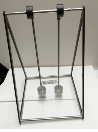
Untreated external examples of other 'simple' machines capable of very complex (chaotic) motion:
Compound pendulum at the US National Center for Atmospheric Research (NCAR) in Boulder, CO.
URL → https://www.youtube.com/watch?v=zvIY1z0xcek
Triple pendulum at the University of Sydney School of Physics in AU
URL → https://www.youtube.com/watch?v=J85gpcjvqzs
(Ch. 5-9 of Unit 2)
Covariant derivative and Christoffel Coefficients Γij;k and Γij;k
Christoffel g-derivative formula
What’s a tensor? What’s not?
General Riemann equations of motion (No explicit t-dependence and fixed GCC)
Riemann-forms in cylindrical polar OCC (q1 = ρ, q2 = φ, q3 = z)
Christoffel relation to Coriolis coefficients
Mechanics of ideal fluid vortex
Separation of GCC Equations: Effective Potentials
Small (nρ:mφ)-periodic and quasi-periodic oscillations
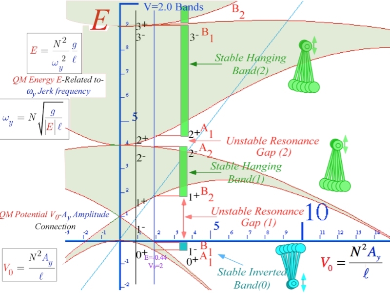
2D Spherical pendulum“Bowl-Bowling” and the “I-Ball”
(nρ:mφ)=(2:1) vs (1:1) periodic and quasi-periodic orbits
Cycloidal ruler&compass geometry
(To be applied to mechanics in electromagnetic fields and collisional rotation in following lectures.)
(Ch. 2.8 of Unit 2)
|
Charge mechanics in electromagnetic fields Vector analysis for particle-in-(A,Φ)-potential Lagrangian for particle-in-(A,Φ)-potential Hamiltonian for particle-in-(A,Φ)-potential Canonical momentum in (A,Φ) potential Hamiltonian formulation Hamilton’s equations Crossed E and B field mechanics Classical Hall-effect and cyclotron orbit and equations Vector theory vs. complex variable theory Mechanical analog of cyclotron and FBI rule Cycloidal ruler&compass geometry Cycloidal geometry of flying levers Practical poolhall application |

This mechanical analog of (Ex,Bz) field mimics A-field with tabletop v-field
|
(Ch. 9 of Unit 3)
Some Ways to do constraint analysis
Way 1. Simple constraint insertion
Way 2. GCC constraint webs
Find covariant force equations
Compare covariant vs. contravariant forces
Other Ways to do constraint analysis
Way 3. OCC constraint webs
Sketch of atomic-Stark orbit parabolic OCC analysis
Classical Hamiltonian separability
Way 4. Lagrange multipliers
Lagrange multiplier as eigenvalues
Multiple multipliers
“Non-Holonomic” multipliers
Cycloid-like curves for rolling constraints
(Ch. 1 of Unit 4)
1D forced-damped-harmonic oscillator equations and Green’s function solutions
Linear harmonic oscillator equation of motion.
Linear damped-harmonic oscillator equation of motion.
Frequency retardation and amplitude damping.
Figure of oscillator merit (the 5% solution 3/Γ and other numbers)
Linear forced-damped-harmonic oscillator equation of motion.
Phase lag and amplitude resonance amplification
Figure of resonance merit: Quality factor q=ω0/2Γ
Properties of Green’s function solutions and their mathematical/physical behavior
Transient solutions vs. Steady State solutions
Complete Green’s Solution for the FDHO (Forced-Damped-Harmonic Oscillator)
Quality factors: Beat, lifetimes, and uncertainty
Approximate Lorentz-Green’s Function for high quality FDHO (Quantum propagator)
Common Lorentzian (a.k.a. Witch of Agnesi)
(Ch. 2-4 of Unit 4 11.12.15)
|
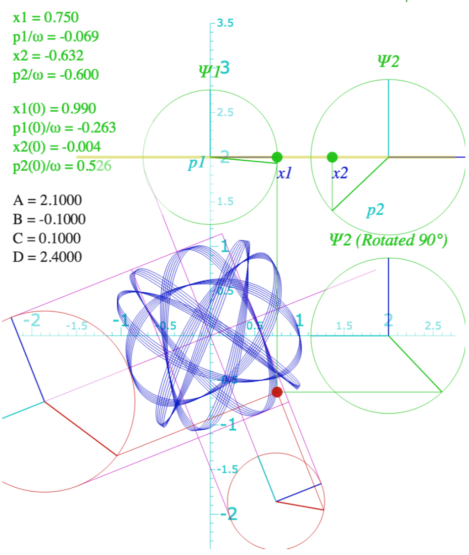
2D harmonic oscillator equations Lagrangian and matrix forms and Reciprocity symmetry 2D harmonic oscillator equation eigensolutions Geometric method Matrix-algebraic eigensolutions with example M = Secular equation Hamilton-Cayley equation and projectors Idempotent projectors (how eigenvalues ⇒ eigenvectors) Operator orthonormality and Completeness (Idempotent means: P·P=P) Spectral Decompositions Functional spectral decomposition Orthonormality vs. Completeness vis-a`-vis Operator vs. State Lagrange functional interpolation formula Diagonalizing Transformations (D-Ttran) from projectors 2D-HO eigensolution example with bilateral (B-Type) symmetry Mixed mode beat dynamics and fixed π/2 phase 2D-HO eigensolution example with asymmetric (A-Type) symmetry Initial state projection, mixed mode beat dynamics with variable phase |
Videos of Coupled Pendula Moderate coupling:
Stronger coupling:
|
(Ch. 2-4 of Unit 4 Ch. 6-7 of Unit 6)
Review: 2D harmonic oscillator equations with Lagrangian and matrix forms
ANALOGY: 2-State Schrodinger: iħ∂t|Ψ(t)〉=H|Ψ(t)〉 versus Classical 2D-HO: ∂2tx=-K•x
Hamilton-Pauli spinor symmetry ( σ-expansion in ABCD-Types) H=ωμσμ
Derive σ-exponential time evolution (or revolution) operator U = e-iHt = e-iσµωµt
Spinor arithmetic like complex arithmetic
Spinor vector algebra like complex vector algebra
Spinor exponentials like complex exponentials ("Crazy-Thing"-Theorem)
Geometry of evolution (or revolution) operator U = e-iHt = e-iσµωµt
The "mysterious" factors of 2 (or 1/2): 2D Spinor vs 3D Spin Vector space
2D Spinor vs 3D vector rotation
NMR Hamiltonian: 3D Spin Moment m in B field
Euler's state definition using rotations R(α,0,0), R(0,β,0),and R(0,0,γ)
Spin-1 (3D-real vector) case
Spin-1/2 (2D-complex spinor) case
3D-real Stokes Vector defines 2D-HO polarization ellipses and spinor states
Asymmetry SA=SZ, Balance SB =SX, and Chirality SC =SY
Polarization ellipse and spinor state dynamics
The "Great Spectral Avoided-Crossing" and A-to-B-to-A symmetry breaking
See also: QTCA Lect. 9(2.12) p.61-103 for polarization ellipsometry
(Classical Mechanics with a BANG! Units 4-6, Quantum Theory for Computer Age - Ch. 10A-B of Unit 3)
(Principles of Symmetry, Dynamics, and Spectroscopy - Sec. 1-3 of Ch. 5 and Ch. 7)
Reviewing fundamental Euler R(αβγ) and Darboux R[ϕϑΘ] representations of U(2) and R(3)
Euler-defined state |αβγ〉 described by Stoke’s S-vector, phasors, or ellipsometry
Darboux defined Hamiltonian H = [ϕϑΘ] = exp(-iΩ•S)·t and angular velocity Ω(φθ)·t=Θ-vector
Euler-defined operator R(αβγ) derived from Darboux-defined R[ϕϑΘ] and vice versa
Euler R(αβγ) rotation Θ =0-4π-sequence [ϕϑ] fixed (and “real-world” applications)
Quick U(2) way to find eigen-solutions for 2-by-2 Hamiltonian H 
|
The ABC’s of U(2) dynamics-Archetypes Asymmetric-Diagonal A-Type motion Bilateral-Balanced B-Type motion Circular-Coriolis… C-Type motion The ABC’s of U(2) dynamics-Mixed modes AB-Type motion and Wigner’s Avoided-Symmetry-Crossings ABC-Type elliptical polarized motion Ellipsometry using U(2) symmetry coordinates Conventional amp-phase ellipse coordinates Euler Angle (αβγ) ellipse coordinates Addenda: U(2) density matrix formalism Bloch equation for density operator |
|
(Ch. 7-8 of Unit 4 11.24.15)
Two Kinds of Resonance: Linear-additive vs. Nonlinear-multiplicative (Parametric resonance)
|
Coupled rotation and translation (Throwing revisited: trebuchet, atlatl, etc.) Schrodinger wave equation related to Parametric resonance dynamics Electronic band theory and analogous mechanics Wave resonance in cyclic symmetry Harmonic oscillator with cyclic C2 symmetry C2 symmetric (B-type) modes Harmonic oscillator with cyclic C3 symmetry C3 symmetric spectral decomposition by 3rd roots of unity Resolving C3 projectors and moving wave modes Dispersion functions and standing waves C6 symmetric mode model:Distant neighbor coupling |
|
C6 spectra of gauge splitting by C-type symmetry(complex, chiral, coriolis, current, ...)
CN symmetric mode models: Made-to order dispersion functions
Quadratic dispersion models: Super-beats and fractional revivals
Phase arithmetic
Algebra and geometry of resonant revivals: Farey Sums and Ford Circles
Relating CN symmetric H and K matrices to differential wave operators
(Ch. 2-4 of Unit 5 12.01.15)
Orbits in Isotropic Harmonic Oscillator and Coulomb Potentials
Effective potentials for IHO and Coulomb orbits Review: “3steps from Hell” (Lect. 7 Ch. 9 Unit 1)
Stable equilibrium radii and radial/angular frequency ratios
Classical turning radii and apogee/perigee parameters ← (A mysterious similarity appears)
Polar coordinate differential equations ← (A mysterious similarity appears)
Quadrature integration techniques
Detailed orbital functions ← (A mysterious similarity appears)
Relating orbital energy-momentum to conic-sectional orbital geometry
Kepler equation of time and phase geometry
Geometry and Symmetry of Coulomb orbits
Detailed elliptic geometry
Detailed hyperbolic geometry
(Ch. 2-4 of Unit 5 11.22.16)
Rutherford scattering and hyperbolic orbit geometry
Backward vs forward scattering angles and orbit construction example
Parabolic “kite” and orbital envelope geometry
Differential and total scattering cross-sections
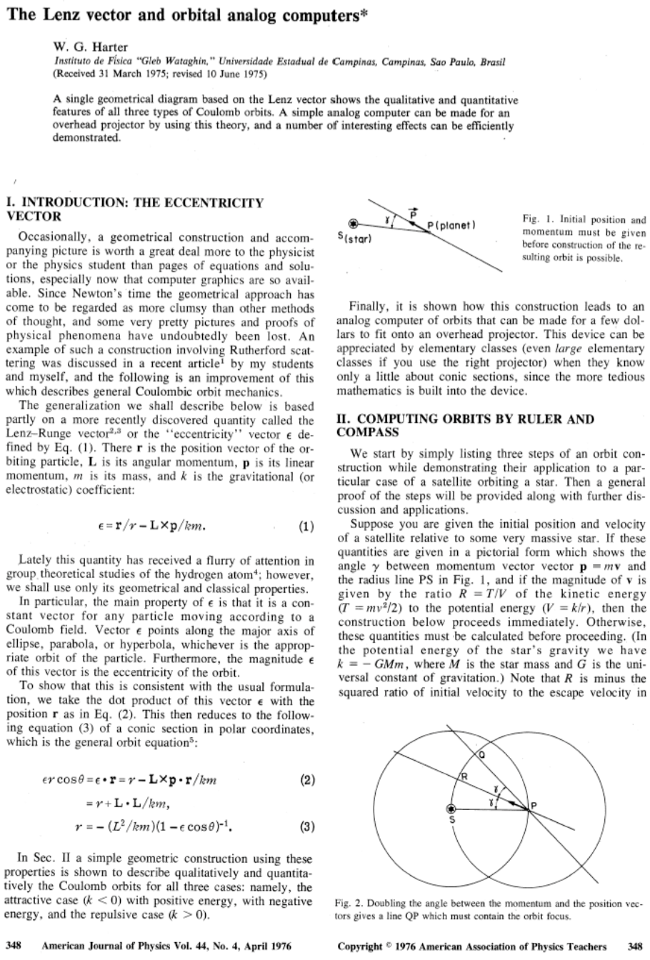
Eccentricity vector ε and (ε,λ)-geometry of orbital mechanics
Projection ε•r geometry of ε-vector and orbital radius r
Review and connection to usual orbital algebra (previous lecture)
Projection ε•p geometry of ε-vector and momentum p=mv
General geometric orbit construction using ε-vector and (γ,R)-parameters
Derivation of ε-construction by analytic geometry
Coulomb orbit algebra of ε-vector and Kepler dynamics of momentum p=mv
Example of complete (r,p)-geometry of elliptical orbit
Connection formulas for (a,b) and (ε,λ) with (γ,R)
(Ch. 2-4 of Unit 5 12.05.15)
Review of Eccentricity vector ε and (ε,λ)-geometry of orbital mechanics ← Review of lecture 26
Analytic geometry derivation of ε-construction ← Review of lecture 26
Connection formulas for (a,b) and (ε,λ) with (γ,R) ← Review of lecture 26
|
Detailed ruler & compass construction of ε-vector and orbits (R = -0.375 elliptic orbit) (R = +0.5 hyperbolic orbit) Properties of Coulomb trajectory families and envelopes Graphical ε-development of orbits Launch angle fixed-Varied launch energy Launch energy fixed-Varied launch angle Launch optimization and orbit family envelopes |
|
(Ch. 2-7 of Unit 6 12.01.16)
2-Particle orbits
Ptolemetric or LAB view and reduced mass
Copernican or COM view and reduced coupling
2-Particle orbits and scattering: LAB-vs.-COM frame views
Ruler & compass construction (or not)
Rotational equivalent of Newton’s F=dp/dt equations: N=dL/dt
How to make my boomerang come back
The gyrocompass and mechanical spin analogy
Rotational momentum and velocity tensor relations
Quadratic form geometry and duality (again)
Angular velocity ω-ellipsoid vs. angular momentum L-ellipsoid
Lagrangian ω-equations vs. Hamiltonian momentum L-equation
Rotational Energy Surfaces (RES) and Constant Energy Surfaces (CES)
Symmetric, asymmetric, and spherical-top dynamics (Constant L)
BOD-frame cone rolling on LAB frame cone
Deformable spherical rotor RES and semi-classical rotational states and spectra
Cycloidal geometry of flying levers
Practical poolhall application
(Ch. 9 of Unit 3)
Some Ways to do constraint analysis
Way 1. Simple constraint insertion
Way 2. GCC constraint webs
Find covariant force equations
Compare covariant vs. contravariant forces
Other Ways to do constraint analysis
Way 3. OCC constraint webs
Sketch of atomic-Stark orbit parabolic OCC analysis
Classical Hamiltonian separability
Way 4. Lagrange multipliers
Lagrange multiplier as eigenvalues
Multiple multipliers
“Non-Holonomic” multipliers
Cycloid-like curves for rolling constraints
(Unit 8 12.06.16)
Learning about sin! and cos and...Trigonometric road maps
Hyper-Trigonometric algebra and phasors in space-time
1CW wavefunctions and phasorsficients and the Lorentz transfor
Per-space-per-time vs Space-time
Wave velocity formulas
Introducing Doppler shifting
Why c is constant?!
Introducing Doppler Arithmetic and rapidity ρ
Optical interference “baseball-diamond” displays phase and group velocity
Details of 2CW wavefunctions in rest frame
Pulse waves (PW) versus Continuous Waves (CW)
Doppler shifted “baseball-diamond” displays Lorentz frame transformation
Analyzing wave velocity by per-space-per-time and space-time graphs
16 coefficients of relativistic 2CW interference
Two “famous-name” coefficients and the Lorentz transformation
Thales geometry of Lorentz transformation
Rapidity ρ related to stellar aberration angle σ and L. C. Epstein’s approach to relativity
Longitudinal hyperbolic ρ-geometry connects to transverse circular σ-geometry
“Occams Sword” and geometry of 16 parameter functions of ρ and σ
Application to TE-Waveguide modes
(Unit 8 12.06.16)
Review: Relawavity ρ functions ⫷⫸ Two famous ones ⫷⫸ Extremes and plot vs. ρ
Doppler jeopardy ⫷⫸ Geometric mean and Relativistic hyperbolas
Animation of eρ=2 spacetime and per-spacetime plots
Rapidity ρ related to stellar aberration angle σ and L. C. Epstein’s approach to relativity
Longitudinal hyperbolic ρ-geometry connects to transverse circular σ-geometry
“Occam's Sword” and summary of 16 parameter functions of ρ and σ
Applications to optical waveguide, spherical waves, and accelerator radiation
Derivation of relativistic quantum mechanics
What’s the matter with mass? Shining some light on the Elephant in the room
Relativistic action and Lagrangian-Hamiltonian relations
Poincare’ and Hamilton-Jacobi equations
Relativistic optical transitions and Compton recoil formulae
Feynman diagram geometry
Compton recoil related to rocket velocity formula
Comparing 2nd-quantization “photon” number N and 1st-quantization wavenumber κ
Relawavity in accelerated frames
Laser up-tuning by Alice and down-tuning by Carla makes g-acceleration grid
Analysis of constant-g grid compared to zero-g Minkowsi grid
Animation of mechanics and metrology of constant-g grid
