MODERN PHYSICS and its Classical Foundations

Unit 1 - Review of Velocity, Momentum, Energy, and Fields

W. G. Harter

Basic ideas of classical velocity, momentum, and kinetic energy (KE) are reviewed using geometry and super-ball collision experiments involving two different masses. The idea of potential energy (PE) and force is introduced by defining PE as the KE of “idler” balls that provide force fields for others. The two most famous PE functions, those of Coulomb and of a harmonic oscillator or linear (Hooke-Law) force are introduced. Elliptic orbit geometry in the latter serves to introduce quadratic forms. This helps derive more advanced ideas of Lagrange, Hamilton, and Poincare and clarifies basic axioms of classical mechanics. A review of complex analysis of functions and fields sets the stage for use in later Units. 

Unit 1 - Table of Contents

	Page in Textbook
Chapter 1. Collision velocity change and slope geometry	21
Idealization and model building	21
Review of slope geometry, sin, sec, tan and complimentary trig functions	23
Slope angles, ratios, and areas	23
Right-handed Cartesian coordinates	25
Change and delta variables	26
Slope and delta ratios	26
Exercises for study of slope and trigonometry	27
Arc functions	29
Know your calculator and ATAN, too! (atan2(y,x))	31
Chapter 2. Velocity and momentum	33
Momentum exchange: a zero-sum game	33
Deducing (perfect?) conservation from (ideal?) symmetry	35
Galilean time-reversal symmetry	35
Galilean relativity and spacetime symmetry	37
Geometry of Balance: Center of Momentum (COM) and Center of Gravity (COG)	38
Chapter 3. Velocity and energy	41
Time symmetry and energy conservation	41
Time symmetry	41
Kinetic Energy conservation	41
Geometry of kinetic energy ellipse and momentum line	42
Introducing vector and tensor geometry of momentum-energy conservation	44
Momentum vs. energy (Bang! for the $buck$!): Standard (mks) units	45
Quick review of kinetic relations and formulas	46
Relations of energy W and space x	46
Relations of momentum P and time t	46
Exercise 1.3.3. Quick construction of Energy ellipses	50
Chapter 4. Dynamics and geometry of successive collisions	51
Independent collision models (ICM)	53
Extreme and optimal cases	54
Integrating velocity plots to find position	55
Help! I’m trapped in a triangle	61
Two balls in 1D vs. one ball in 2D	61
Angle of incidence=Angle of reflection (or NOT)	61
Bang force	61
Kinematics versus Dynamics	62
Dynos and Kinos: Classical vs. quantum theory	62
Chapter 5 Multiple collisions and operator analysis	65
Doing collisions with matrix products	65
Rotating in velocity space: Ticking around the clock	67
Statistical mechanics: Average energy	68
Bonus: Rational right triangles	69
Reflections about rotations: It’s all done with mirrors	69
Through the clothing store looking glass	70
Chapter 6 Introducing Force, Potential Energy, and Action	75
MBM force fields and potentials	75
Isothermal model force laws	76
Adiabatic model force laws	77
Conservative forces and potential energy functions	77
Is it +or-? Physicist vs. mathematician and the 3rd law	77
Isothermal “Robin Hood”and “Fed rules”	78
Oscillator force field and potential	79
The simplest force field F=const.	81
Introducing Action. It’s conserved (sort of)	81
Monster mass M1 and Galilean symmetry (It’s deja vu all over, again.)	82
Chapter 7 Interaction Forces and Potentials in Collisions	87
Geometry of superball force law	87
Dynamics of superball force: The Project-Ball story	88
The trip to Whammo	88
Eureka! Polka-dots save Project Ball	88
The “polka-dot” potential	89
Force geometry: Work and impulse vs. energy and momentum	91
Kiddy-pool versus trampoline	91
Linear force law, again (But, with constant gravity, too)	93
Why super-elastic bounce?	95
RumpCo versus Crap Corp	95
Seatbelts and buckboards	97
Friction and all that “dirty” stuff	98
Chapter 8 N-Body Collisions: Two’s company but three’s a crowd	101
The X3: Three-ball towers	101
Geometric properties of N-stage collisions	103
Supernovae super-duper-elastic bounce (SSDEB)	103
Newton’s balls	103
Friction, again: Inelastic energy-momentum quadratic equations	105
Geometric derivation of elastic and inelastic energy ellipses	107
Ka-Runch-Ka-Runch-Ka-Runch-Ka-Runch-...:Inelastic pile-ups	109
Ka-pow-Ka-pow-Ka-pow-Ka-pow-...:Rocket science	111
Chapter 9 Geometry and physics of common potential fields	115
Geometric multiplication and power sequences	115
Parabolic geometry	117
Coulomb and oscillator force fields	119
Tunneling to Australia: Earth gravity inside and out	121
To catch a falling neutron starlet	123
Starlet escapes! (In 3 equal steps)	125
No escape: A black-hole Earth!	125
Oscillator phasor plots and elliptic orbits	126
Chapter 10 Calculus of exponentials, logarithms, and complex fields	131
The story of e : A tale of great interest	132
Derivatives, rates, and rate equations	134
The binomial expansion	135
General power series approximations	137
Sine-wave power series	139
Euler’s theorem and relations	141
Wages of imaginary interest: Phasor oscillation dynamics	142
What Good Are Complex Exponentials?	143
Complex numbers provide "automatic trigonometry"	143
Complex exponentials Ae-i_t tracks position and velocity using Phasor Clock	143
Complex numbers add like vectors	143
Complex products provide 2D rotation operations	144
Complex products set initial values	144
Complex products provide 2D “dot”(•) and “cross”(x) products	144
Complex deriviative contains “divergence”(_•F) and “curl”( _xF) of 2D vector field	145
Complex potential _ contains “scalar”( F= __) and “vector”( F=_xA) potentials	145
Complex integrals ∫ f(z)dz count “flux”( ∫Fxdr) and “vorticity”( ∫F•dr)	146
Complex derivatives give 2D multipole fields	151
Complex power series are 2D multipole expansions	152
Complex 1/z gives stereographic projection	154
Cauchy integrals	156
Chapter 11 Oscillation, Rotation, and Angular Momentum	159
Keplerian construction of elliptic oscillator orbits	159
Elementary ellipse construction	159
Orbiting versus rotating: Centripetal versus centrifugal	161
Circular curvature	162
More inertial forces: Coriolis and tidal forces	163
Vector analysis and geometry of elliptic oscillator orbit	165
Matrix operations and dual quadratic forms	166
Slope multiplication and eigenvectors	167
Geometric slope series	168
Angular momentum and Kepler’s law	170
Flight of a stick: Introducing geometry of cycloids	170
Center of percussion, radius of gyration, and “sweet-spot”	171
Chapter 12 Velocity vs momentum functions: Lagrange vs Hamilton	175
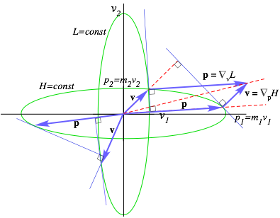
Relating energy ellipses in velocity and momentum space	175
Lagrangian, Estrangian, and Hamiltonian functions	175
L, E, and H ellipse geometry	176
Legendre contact transformations	178
Extreme geometry of contact transformations	179
General contact transformation geometry	180
The Equations of the Classical Universe (Lagrange, Hamilton, and others)	183
Lagrange’s version of Newt-II (f=Ma)	185
Hamilton’s version of Newt-II (f=Ma)	188
Variational calculus of Lagrangian mechanics	189
Poincare’s invariant, quantum phase, and action	190
Huygen's principle: "Proof" of classical axioms and path integrals	190
Bohr quantization	193
Appendix 1A Vector product geometry and Levi-Civita _ijk	1
Determinants and triple products	2
Operator products	3
Unit 1 References	1

-Unit 1 - Review of Velocity, Momentum, Energy, and Fields

Perhaps the most common fundamental modern physics experiment is to collide particles against each other. That’s all they do at LHC (Large Hadron Collider) where protons are rammed head-on at speeds above 0.999999c at several TeV (Trillion or Tera-electron Volts). Electron microscopes and laser spectral experiments are just particle crashes, too, involving molecules, atoms, electrons, and photons at intermediate energies ranging from keV (Thousand or kilo-eV) to about 1eV for one green light photon down to ultra-low energies measured in neV (Billionths or nano-eV) for collisions in BEC experiments. We begin studying momentum and energy by making classical analogies to common (I hope not for us!) freeway car crashes.

Chapter 1. Collision velocity change and slope geometry

Ka-runch! A 4-ton SUV going 60mph rear-ends a 1-ton VW going 10mph. See Fig. 1.1a. The SUV driver was busy texting a cell-phone and not watching the road. Both vehicles abruptly change speeds as seen in Fig. 1.1b-c. In order to calculate the speed changes we need to decide whether our collision is a “ka-runch!” where the cars get welded into a single mass as in the top right of Fig. 1.1(c) or a “ka-bong!” where they bounce off with no damage (very unlikely) as in center Fig. 1.1b or else quite likely intermediate “ka-whump!” collisions to be detailed later on. The technical term for ka-runch is a totally inelastic collision. We’ll study it first followed by ka-bong, or technically a perfectly elastic collision, and finally the generic range of ka-whumps or inelastic collisions that lie between the first two ideals or extremes.

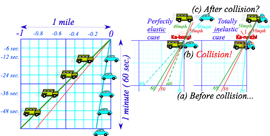
Fig. 1.1 Time vs. space graphs of (a) SUV (going 60mph) and VW (going10mph), (b) collision, and (c) possible outcomes of two extreme cases: the inelastic “ka-runch!” and perfectly elastic “ka-bong!”

This text uses of geometry to get quicker results and expose logic. First, let’s review some conventions regarding slope on graphs. Our first graph (Fig. 1.1 or Fig. 1.2a below) is a time vs. distance plot and speed is slope-from-vertical as favored in relativity theory and by Einstein’s math teacher, Herman Minkowski. In contrast, Newtonian calculus favors distance vs. time plots like Fig. 1.2b and speed is slope-from-horizontal. Both our plots are scaled so a 1:1 ratio (45°slope=1/1) represents 60 mph = 1 mile/min. in Fig. 1.2a or 1 min./mile in Fig. 1.2b. Plot (a) compliments (b). One becomes the other by doing a mirror-reflection across the 45° diagonal (1:1)-“SUV-line” that is the same in (a) and (b). Plot (a) is best for car motion since cars go horizontally. For (b) one might ask, “Do cars climb walls?!” (See review of slope.)

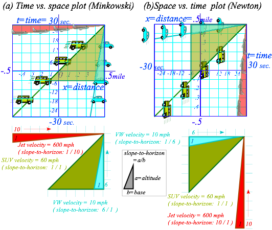
Fig. 1.2 Complimentary plots  (a) Minkowski time vs. space plots vs. (b) Newton’s space vs. time plots.

            Before proceeding with car-crash analysis, it is required we give full disclosure of an important part of physics that concerns its idealization and model building.

Idealization and model building

Landscape 1.1 below applies explicitly to this Unit 1 but implicitly to this entire text and to all other physics texts. Scientific theory always requires an idealized model in which to develop its axioms and logic for its qualitative and quantitative thought (Gadaken) experiments. It’s an ancient tradition for physics.

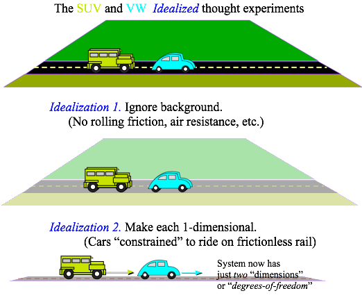
Landscape 1.1 Idealized model for collision model and thought experiments

Here is where we play “Let’s pretend.” We ignore most of the reality of the open road, most notably friction of the road surface-tire interface and air resistance. Also, we restrict the number of independent variables or dimensions. They are also called degrees of freedom. Here there is only one dimension for each car or two dimensions in all. It is as though we have re-framed the car crash as a perfect air-track with two bumper-cars floating on it. Models like this one are meant to be expanded. The next Landscape 1.2 begins this process by listing the most important classical degrees of freedoms for AMO physics.

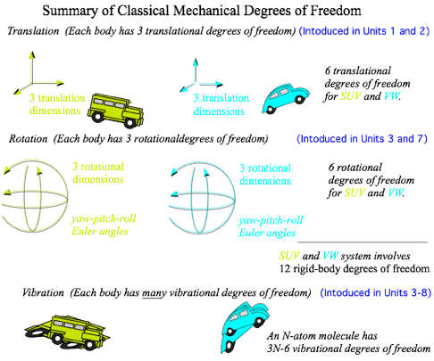
Landscape 1.2 Some idealized classical model degrees of freedom

Models of molecules, atoms, and even nuclei begin with classical models having 3 translational, 3 rotational, and N vibrational degrees of freedom for every nucleon or nucleus and every electron in them.

Classical translation-rotation-vibration degrees of freedom may be expressed in coordinates that are more convenient than the Cartesian coordinates (CC). These are known as Generalized Curvilinear Coordinates (GCC) and are essential in general relativity theory. A simple example, polar coordinates, are used to introduce GCC in Chapter 12. Other examples of Orthogonal Curvilinear COordinates (OCC) are derived in Chapter 10 in connection with complex field coordinates.

In quantum mechanics, we find for each classical degree of freedom an infinite number (∞) of degrees of freedom. In fact, it’s two infinities (2∞) for each since they are complex dimensions.

Now if you know everything about slope, you may proceed to Ch. 2 for more news on the car crash. But, there are some tricky and subtle things in this Review of slope... section that follows. These could bite you later! So it is definitely recommended reading. See if you can do exercises without peeking at answers.
Review of slope geometry, sin, sec, tan and complimentary trig functions

Slope is defined as the ratio Äy/Äx of vertical altitude Äy per horizontal base Äx. This equals velocity v=Äx/Ät for a horizontal time-t-axis and vertical space-x-axis like Fig. 1.2b. So horizontal x-axis and vertical time-t-axis of Fig. 1.2a has slope=Ät/Äx=1/v inverse to Fig. 1.2b slope. The lowest slope=1/10 in Fig. 1.2a belongs to jet velocity v=600mph that is the highest slope=10/1 in Fig. 1.2b, and a low VW velocity of v=10mph has a steep triangle of slope=6/1 in Fig. 1.2a but in Fig. 1.2b that VW line is a low slope=1/6.

Each unit graph square in Fig. 1.2a has a horizontal scale factor of s_x=0.1mile(per square) and a vertical scale factor of s_y=6sec.(per square) and vice versa for Fig. 1.2b. If you multiply scale s_x by factor f_x and s_y by f_y then each graph slope =(n_y vert. squares)/(n_x horiz. squares) changes to (f_x/f_y).

We do rescaling of dimensions to change units. For example, changing miles to feet in Fig. 1.2a uses factor f_x =5,280 ft. per mile (or ) and changing minutes to seconds uses f_y =60. The scale ratio (f_x/f_y) is 88, that is, 60mph equals 88 . SUV slope of 1 in Fig. 1.2b is 88 in a ft. vs. sec. plot. That’s too high to plot 60mph accurately but a ft. vs. sec. or ft. vs. min. plot will be more appropriate for parking lot speeds.

Slope angles, ratios, and areas

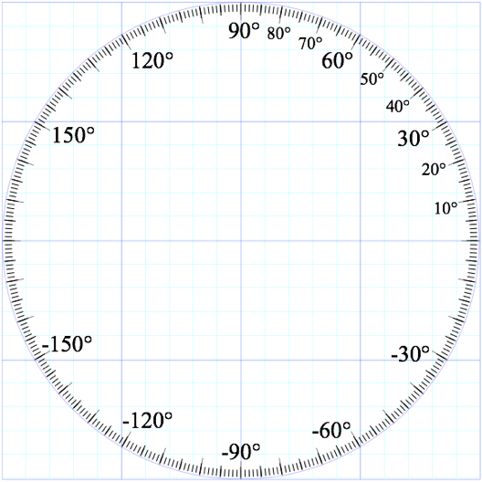
            Most of us learn to measure slope by degrees(°) of a slope angle ó. Greek “s” or sigma ó stands for sector slope. (We also use theta (è) or phi (ö).) But, degrees are an arbitrary choice of 180° per (1/2)-turn or 360° per full turn. A better unit is 1 radian=180/π~57.3°. A ó=1radian-sector on unit circle (r=1) (Fig. 1.3a) has unit arc-length (l=ó·r=1) and unit sector area (A=ó·r²=1) based on π=3.14159…(pi), not an arbitrary number.

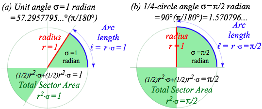
Fig. 1.3 (a) Definition of unit angle (ó =1) on unit circle (r =1) (b) A quarter turn sweeps half the area.

            The trick here is that the sector slope line sweeps out two pieces of the pie to make a whole pie or area pi=π if angle ó is π or 180°. The 1/4-circle angle ó=ð/2 in Fig. 1.3b sweeps area πr²/2=π/2 of half a pie. It may not be how you serve pie, but it’s how mathematicians serve π. (There (or their) pie (or pi) are squared!)

Actual slope is the tangent of angle ó written tanó and so called since it is the length of a line tangent to or “touching” a unit circle from angle ó to x-axis. (See Fig. 1.4b.) Another triangular ratio is the sine or sinó that stands (I’m guessing) for “slope over incline.” The tangent in Fig. 1.4 is an a:b ratio (), but the sine is an a:r ratio () that civil engineers use to “grade” roads.

percent-grade=100·(altitude Äy gained)/(distance Är traveled) =100 sin ó

High grades are good in school but bad for roads. An interstate highway would “flunk” anywhere its grade was above 5%. This changed in 2001 with the Bush administration’s “No Road Left Behind” policy.

Each triangle ratio switches places with its codependent ratio if you switch x-and-y-axes (or altitude-and-base) or switch Fig. 1.2a Minkowski plots to Fig. 1.2b Newton plots. For example, a cotangent ratio is codependent to tan ó, and cosine ratio  is codependent to sin ó.

In comparing (a) vs. (b) in Fig. 1.2 we saw that a slope (like 6/1) in (a) is inverse slope (1/6) in (b). (That was for the 10mph VW.) In other words, any slope in (a) becomes  in (b). Also any slope angle ó in (a) becomes a compliment to angle ó in (b). (See Fig. 1.4a.)

From the two preceding paragraphs we deduce that any ratio like sinó or tanó for angle ó must equal its co-ratio for the compliment ó_c=ð/2−ó, and vice versa.

Two other ratios use secant (or “sword-like”) lines that pierce the circle in Fig. 1.4b. The horizontal line is a secant ratio  and its co-ratio is a cosecant ratio .

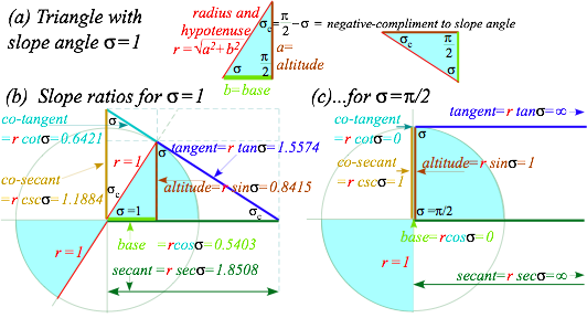
Fig. 1.4 (a) Right triangle geometry for ó=1 slope (b) Triangle ratios for ó=1 and (c) ó=ð/2.

Right-handed Cartesian coordinates

Rene Descartes (1596-1650) is said to have invented (or discovered) the Cartesian graph and coordinate system. We usually call the two-dimensional (2D) version “XY-coordinates” and three-dimensional (3D) versions are “XYZ-coordinates.”

Four-dimensional (4D) space-time (xyzt)-Minkowski coordinates after Herman Minkowski (who was Einstein’s math professor)^†came later (1905-1908). The 2D projection of one space dimension (x or y or z) and time scale-by-lightspeed (ct) is called a Minkowski graph. Lightspeed c=2.99792458 m/s has velocity units so ct has distance units like x or y or z.

Two-dimensional (2D) XY-graphs often draw the primary X or x-axis along the horizontal direction with x increasing to the right, and then place the secondary Y or y-axis perpendicular or normal to the X-axis with y increasing vertically.

What (or which) physics variables should be “primary?” Well, that’s up to you. The choice between Minkowski(a) and Newton(b) in Fig. 1.2 is a matter of taste.

The graph above is called a right-handed coordinate system since it points like your thumb (X) and forefinger (Y) of your right hand as you extend to shake hands or hand someone a plate of escargot. (Descartes’ French cuisine is respected here.)

A toothpick sticking up from the escargot points in the Z or z-axis direction of a right-handed 3D Cartesian coordinate system as shown below.

† Minkowski (who was Polish) told Einstein (who was Swiss) that he was a “fat lazy boy.” Einstein was so insulted that he never used Minkowski plots. It is sad story since Herman’s graphs could have helped many more to visualize relativity by exposing its geometric structure. Eventually, we hope to make up for that sad mistake!

A. Einstein, Annalen der Physik 17, 891(1905).

H. Minkowski, Mathematisch-Physikalische Klasse, vol. 1, 53 (1908).

Change and delta variables

The delta notation, such as Äx, Äv, Ät, and so forth, is confusing to one who has not had a calculus course (or has forgotten that stuff). Roughly speaking, the Greek upper case “D” or delta (Ä) stands for “difference” or differential, and Äx should be read as “change of x” or differential of x and thought of as a single entity.

It is a common mistake to read  Äx as “Ä multiplied by x” or “Ä times x ” since, after all, product p of quantities a and x is written p=ax or better p=a·x. Instead, the mathematical cognescenti think of Ä as an operation that acts on a variable x or whatever to give whatever change has occurred in that variable.

When the letter Ä is used to denote an actual number or variable one should take care to write its product with another variable x as Ä·x or (better) x· Ä to avoid confusing it with Äx.

Slope and delta ratios

Slope ratio Äy/ Äx of a line or of a triangular hypotenuse is a key concept that is common to mathematics and physics beginning with Babylonian and Greek plane geometry of Euclid (300 BCE), and progressing through analytic geometry of Descartes (1620), the complex trigonometry of Euler (1700), the calculus of Newton (1720), the relativity of Einstein (1905), and the quantum mechanics of Planck (1900), Bohr (1920), Schrodinger (1925), and Dirac (1930). (That’s a short list. A full one could take pages.) Physics uses slope like soup uses water. It’s all based on slope and related triangular angles, areas, and ratios. We must study slope!

So far we have only talked about slope of straight lines in Fig. 1.1-2. For them triangle size or location makes no difference to ratio Äy/ Äx. All triangles in the figure (a) below are similar triangles, but triangles hanging on a curve in figure (b) are not.

Slope of a triangle hanging on a curve depends on location x and base segment size Äx. Soon we will define slope of a tangent line to a curve in (b) by making its base segment Äx so small that the curve over it looks straight as in (a). Then tangent slope (to graph accuracy) only depends on location x on the curve and not on tiny Äx.

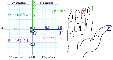
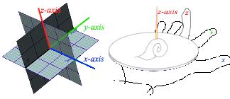
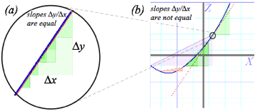
            Fig. 1.4b has eight different but similar triangles with the same angles (ó,ð/2,ó_c) as the triangle in Fig. 1.4a. Can you spot them? Whether big or small, similar triangles share ratios (sine, cosine, or tangent) if (and only if) they share angles. To do geometry problems we look for “hidden” similar triangles and hidden right triangles that form similar rectangles. Right triangles have relation a²+b²=r² of Pythagoras (~570 BC).

            One secret is to visualize sequences of scale change or rotation transformation as in Fig. 1.5 where each rectangle is rotated by 90° and shrunk by a factor cotó=64.2%. Rectangle diagonals in Fig. 1.5a (and sides in Fig. 1.5b) give a power sequence (…tan¹ó,tan⁰ó=1,(tanó)^-1=cot¹ó,(tanó)^-2=cot²ó,(tanó)^-3=cot³ó,…).

            A power sequence is also called a geometric sequence since it is suggested by geometry. A rectangle sequence in Fig. 1.5a is lined up with the XY coordinates of the page, that is, each side has zero or infinite slope but the first diagonal (tanó) has a negative slope angle of -ó_c = –1-radian or –57.3°. The sequence in Fig. 1.5b begins with a rectangle side (tanó) at angle –57.3°. Each sequential rotation in either figure is 90° clockwise around the original tangent point with rectangle size shrunk by factor cotó=64.21% each time.

Fig. 1.5 Geometric cotó=0.6241 sequences of whirling rectangle segments based on slope angle ó=1.

Exercises for study of slope and trigonometry

1. Construct whirling square diagrams for 60° slope angle ó=ð/3 without using protractor. First compare the precision of graph-derived values of sinó,  cosó, tanó , etc. with algebraic ^and/_or calculator-derived numbers.

Solution Hints:

Only certain angles have exact Euclid rule&compass construction and ó=60° is one of them. (But, ó=1 isn’t!) If you could “straighten” the (l=1)-arc of a (ó=1)-sector (Fig. 1.3a) to one (r=1)-side of an equilateral triangle, its slope angle would grow from ó=1=57.3° to ó=π/3=60° as shown in Fig. 1.6b.

To construct a 60° slope a′ la Euclid, draw a radius-(r=1) circle by compass and use the same radius-r setting to strike an arc from X point-(x=1,y=0) to locate R as in Fig. 1.6b. So now, theoretically, arc-RX is l=π/3=1.0472…long approximately but line-RX has length-(r=1) exactly. At 2-figure precision both have length 1.0, but at 3-figure precision, arc-RX length is 1.05, 5% greater than line-RX length 1.00.

Whether a math or physics theory is “correct” or not depends on our level of precision. As we will see, it is pretty tough to get order-3 absolute precision (1 part in 1,000) with ruler and compass construction but order-2 is pretty easy. By taping fishing line onto arc-RX, we can see that it is about 5% shorter than a unit line, but measuring 4.7% is challenging and 4.72% requires tools most don’t have.

We easily get level-9 precision by poking sin(π/3) into a calculator (or sin60° if set for degrees)  to get sin(π/3)=0.866025403…. but only can estimate 0.86 or 0.87 in Fig. 1.6b graph as indicated by ??? marks.

To construct the tangent declination by compliment angle ó_c= π/2-π/3= π/6 (or 90°-60°=30°) we strike a unit arc off the –Y point to intersection point Q on the 4^th quadrant-YQX of unit circle in Fig. 1.6c. The line OQ thru point Q is perpendicular or normal to original slope line OR since ó_c+ó is π/2(90°) for any ó.

This line OQ drawn thru point R is the tangent decline we need for this problem. Just redo arc inter-sector -YQO to make sector NPR centered at R instead of O. Then draw tangent line PR so it extends down to secant point S on the X axis and up along the cotangent line to the cosecant point on the Y axis.

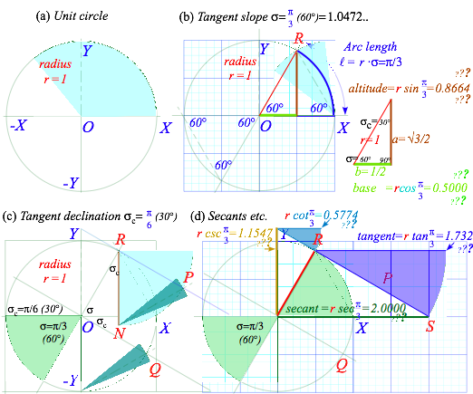
Fig. 1.6 Details of a geometric construction of Fig. 1.5 for slope angle ó=ð/3 (60°)

            Segments OS and YR provide numerical estimates of calculated values sec(π/3)=2.000 and csc(π/3) =1.155 along X and Y axes, respectively, in Fig. 1.6d. The value sec(π/3)=2 like its inverse cos(π/3)=1/2 is exactly rational, a nice feature of a (30°,60°,90°)-triangle with side ratios (b:a:r)=(1:√3:2) (It is a right triangle, so: a²+b²=r².) The “30-60” is a famous right triangle students must learn. Others are “3-4-5” ((a:b:r)=(3:4:5)) and the “45” ( (45°,45°,90°)or(a:b:r)=(1:1:√2)). A “Golden” ratio  triangle is very cool (and rich).

Arc functions

So far we give an angle or unit-circle arc ó and construct or calculate trigonometric functions of ó including a=sin ó, b=cos ó, t=tan ó, 1/a=csc ó or their co-functions. Now consider the reverse or inverse case: we are given a, or b, or t etc. and must come up with an arc ó (or arcs ó₁, ó₂...) that gives a, etc. To do this we find arc-functions arc-sine, arc-cosine… or inverse trig functions sin^-1, cos^-1…as follows.

ó =arcsin(a)=sin^-1(a), ó =arccos(b)=cos^-1(b), ó =arctan(t)=tan^-1(t),…

The exponential (^-1)-notation seems to confuse sin^-1(a) with (sin(a))^-1=1/(sin(a)) that we do not want here. (However, it is conventional to write (sin(a))ⁿ=sinⁿ(a) or any power but (^-1).)

            Algebra of arc-functions is trickier than algebra of functions themselves. Geometric constructions of sin^-1, cos^-1…etc. are not so tricky but quite simple and revealing. To find sin^-1(0.5), for example, we draw a horizontal line at y=0.5 and see where it intersects the unit circle. (Fig. 7a) Nothing to that! Except, we see there are two angles ó₁=π/3 and ó₂=2π/3 that give sinó₁=0.5=sinó₂. The same applies to cos^-1(0.5) except now the angles are ±π/3. (Fig. 1.7b) Note the antipodal (±180°) angles that equal tan^-1(0.5). (Fig. 1.7c)

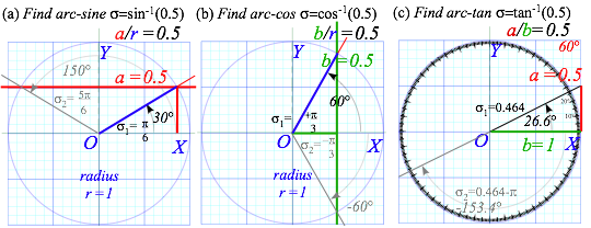
Fig. 1.7 Geometric construction of arc-trig functions of 0.5=. (a) sin^-1()  (b) cos^-1()  (c) tan^-1()

2. Find arc-secant (say, sec^-13.0) by geometry. Try it first without looking at the answer.

Solution Hints:

We need to find the tangent that goes from 3.0 to touch the circle. A circle of radius r=3.0 concentric to the unit circle has rectangle tangents of that size that we copy from x=3.0 to touch unit circle.

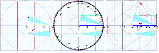
Fig. 1.8 Geometric construction of arc tangent, arc secant, and geometric-mean square-root.

Or else we simply draw rectangle diagonal thru unit circle. This involves Thales’s Geometric Mean (GM) construction in Fig. 1.9a of a product square root √(a·b). In Fig. 1.8 it is √8=2.82… the desired tangent. The special case of the Golden Mean is shown in Fig. 1.9b. The whirling rectangle in Fig. 1.5 is a whirling square in Fig. 1.10 if the rectangle tangent and cotangent are Golden Means 1.618.. and 0.618.., respectively.

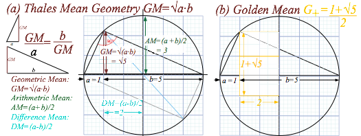
Fig. 1.9 Thales construction of geometric-mean, square-root, and Golden Mean.

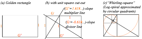
Fig. 1.10 (a) Golden Rectangle, (b) Golden slope geometry, and (c) Whirling Square like Fig. 1.5.
Know your calculator and ATAN, too! (atan2(y,x))

Scientific calculators do not always give the solution you want for arc-function sin^-1(a), cos^-1(b), or tan^-1(b/a). For one thing, they never give an angle in the 3^rd quadrant (minus-x,minus-y) so you could be wrong at least 25% of the time.

But it is worse than that. “Blind” arc-calculations are wrong half the time.

As you vary altitude a=y from (+1) to (−1) values in Fig. 1.7a the 1^st arc-solution ó₁= sin^-1(a/r) sweeps the unit circle in the right-half plane while its x-reflection is the 2^nd solution ó₂ is in the left-half plane. The calculator ignores ó₂.

As you vary base b=x from (+1) to (−1) values in Fig. 1.7b the 1^st arc-solution ó₁= cos^-1(b/r) sweeps the unit circle in the upper-half plane while its y-reflection is the 2^nd solution ó₂ is in the lower-half plane. Again, the calculator ignores ó₂.

Varying either altitude a=y or base b=x from (+1) to (−1) in Fig. 1.7c gives a full range of solutions ó₁= tan^-1(a/b) but a calculator cannot distinguish between the first solution and the 2^nd antipodal solution ó₂= tan^-1(-a/-b) since a/b=-a/-b.

So the calculator plays it safe and gives the acute angle solution in the arc-range –90° and +90°, that is . The obtuse angle solution is ignored for ranges +90° to +180°  or -90° and -180°

A correct solution is the sure-fire atan2(y,x) function that requires you to give both the altitude a=y and the base b=x (with correct signs, of course) so it knows which quadrant you’re in. The atan2, built into calculators gives what is called the rect-to-polar coordinate conversion often labeled by a -button.

 Plug in x and y and out comes and . The è is our ó.

Trig function plotting exercises (And, how we trisect angles)

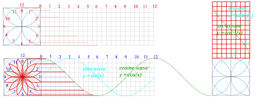
3. Use ruler&compass to plot y=cos(x) and y= cos^-1(x)=arccos(x). Do y=sin(x) and y=sin^-1(x). Begin by constructing a 12-pt “clock” circle. Repeat using 45° diagonals to make a 24-hr clock and project the 24 points horizontally for y=cos(x) and vertically y=cos^-1(x)=arccos(x). Shift plot by 3 hours (90°) for sine and arc-sine functions. Each “hour” is angle 15° or π/6. Sine curves allow “forbidden” constructions such as cycloids and angle-n-sections. In quantum physics sinusoidal waves are really important curves!

Exercise 1.1.4

Construct both Golden angles associated with the Golden Ratios G₊ and G_-  and measure their slopes in degrees on protractor graph paper below. (Also available online.) Can you find a simpler (Pythagorean) construction of √5 ?

Exercise 1.1.5

 Construct whirling rectangle diagram like Fig. Fig. 1.5 but for Golden slope angle to give whirling square sketched in Fig. 1.10. Use protractor graph from Ex. 1.1.3 to measure angles of slopes obtained this way.