Chapter 3. Velocity and energy
We noted that reflection symmetry or balance in space is connected with momentum or P=m·V conservation. Uniformity or “sameness” of coordinate and velocity space means the SUV can lose a unit of momentum only if the VW gains that unit, and vice versa. Momentum is a zero-sum game that does not depend on whether the two protagonists bounce elastically or crumple in-elastically during their collisions.
Time symmetry and energy conservation
Now we consider symmetry or balance in time. This is connected with a something called energy that also plays a conservation zero-sum game but, unlike momentum, requires elastic (Ka-Bong!) collisions. While momentum conservation is axiomatic, energy conservation is derived by algebra or geometry. Let’s do that.
Symmetry
balance in Fig. 2.6 is between pairs of velocity values (VSUV,VVW)
or spatial coordinates
(xSUV,xVW) of the colliding SUV and VW. Weighted
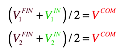
average (2.5b) equals the same VCOM
for the initial pair ![]() ,
the final pair
,
the final pair ![]() ,
or a pair
,
or a pair ![]() at
anytime t. (Recall (2.1) and
(2.5), too.)
at
anytime t. (Recall (2.1) and
(2.5), too.)
![]() (3.1)
(3.1)
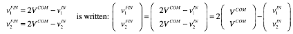
We subtract IN’s from FIN’s to isolate SUV terms from VW terms and redo zero-sum relation (2.3).
![]() (3.2b)
(3.2b)
(Ch.1 reviews Delta notation![]() .) Here is
another way to write the zero-sum relation.
.) Here is
another way to write the zero-sum relation.
![]() (3.3)
(3.3)
Now
consider balancing IN
vs. FIN pair ![]() for SUV or
for SUV or ![]() for VW. Elastic (Ka-Bong!) cases in
Fig. 2.2 or Fig. 2.6 show how VCOM is a balanced IN-vs.-FIN pair-average of both SUV and VW.
for VW. Elastic (Ka-Bong!) cases in
Fig. 2.2 or Fig. 2.6 show how VCOM is a balanced IN-vs.-FIN pair-average of both SUV and VW.
![]() (3.4)
(3.4)
This is an algebraic statement of a time reversal symmetry axiom or IN vs. FIN balance mentioned earlier. For ideal elastic (Ka-Bong!) collisions, IN and FIN points balance around the COM point. Switching past and future gives a similar Ka-Bong and not a miraculous “un-crash” where VFIN ends up further from VCOM than VIN was.
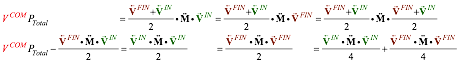
A definition of energy emerges from multiplying space and time balance equations (3.3) with (3.4)
![]() (3.3)·(3.4)
(3.3)·(3.4)
Then adding the (-)-terms to both sides isolates IN-terms. A FIN-sum is proved to equal an IN-sum.
![]() (3.5a)
(3.5a)
This derives a second quantity 1/2M·V2 (or just M·V2) whose conserved sum is assured by the axiom (2.5a) (conserved sum of momentum M·V) and t-reversal axiom (3.4). (M·V is conserved by x-reversal symmetry.)
This 1/2M·V2 is kinetic energy (KE) and it is conserved by a relation like (2.5a) for momentum P=M·V.
![]() (3.5b)
(3.5b)
![]() (2.5a)repeated
Conservation holds for any overall factor so the factor-1/2 in
(3.5a) looks fortuitous. But, KE
is defined later by integral
(2.5a)repeated
Conservation holds for any overall factor so the factor-1/2 in
(3.5a) looks fortuitous. But, KE
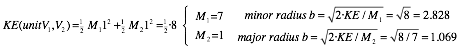
is defined later by integral![]() or area KE=1/2
or area KE=1/2![]() =1/2M·V2 of a
triangle with base P=M·V and altitude V. Thus (3.3)·(3.4)
is product
=1/2M·V2 of a
triangle with base P=M·V and altitude V. Thus (3.3)·(3.4)
is product ![]() =1/2M·V2 of
=1/2M·V2 of ![]() and V-average
and V-average ![]() . Fig.
3.1 below also verifies the 1/2.
. Fig.
3.1 below also verifies the 1/2.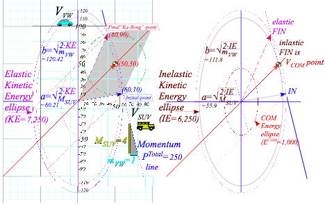
Fig. 3.1 Elastic KE-ellipse hits (PTotal)-line at IN and FIN pts. Inelastic IE-ellipse hits only at VCOM pt.
Geometry of kinetic energy ellipse and momentum line
First, P-conservation relation (2.5a) is rearranged to show its geometry.
The VSUV-vs-VVW-plot of (3.6a) in Fig. 3.1 is a line of slope –MSUV/mVW thru the COM-point (VCOM ,VCOM).
y-y0=m·(x-x0)
where: ![]() and:
and:
![]() (3.6b)
(3.6b)
Then KE conservation relation (3.5a) is rearranged by placing KE and masses into denominator.
![]() becomes:
becomes:
 (3.7a)
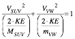
The VSUV-vs-VVW-plot (3.7a) in Fig. 3.1 is KE-ellipse (3.7b) of x-radius a and y-radius b to match (3.7a).
![]() where:
where: 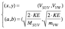 (3.7b)
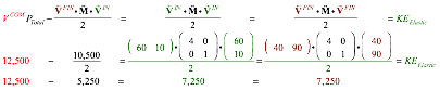
Fig. 3.1 also shows an inelastic Ka-runch-IE-ellipse inside and a small KE-ellipse seen in the COM-frame. Elastic KE (VSUV=60, VSUV=10), inelastic IE(50, 50), and ECOM(10, 40) in COM frame is worked out for Fig. 3.1.
![]()
![]()
![]() (3.8)
(3.8)
The difference in energy between the two extreme types of collision, Ka-Bong and Ka-runch, is 1,000 units in the Earth frame and 1,000 units in the COM frame. But, only in the COM frame does the Ka-runch! take all the kinetic energy and leave both cars standing still. Galilean symmetry has “cost” of damage be the same in all frames. A generic Ka-whump will only lose some fraction of ECOM=1,000 inelastic crumpling.
A
fine point of Fig. 3.1 geometry deserves notice. The tangent slope to the IE-ellipse at
pt-(50, 50) on the 45°(slope-1)-COM-line is
that of the momentum line, namely –MSUV/mVW=-4.
Conversely, slope of dashed tangent lines to the ECOM(10,
40)-ellipse on (slope=-MSUV/mVW)-line
is that of the COM–line, namely slope-1. This beautiful duality is
an important part of mechanics, both classical and quantum. Here it has IN and FIN points
stay on a (slope=-MSUV/mVW)-line
even as they coalesce to a
tangent point of non-collision! Head-on ![]() collisions are
plotted in Fig. 3.2 below showing increasing inelasticity in parts (b) and (c).
(These involve a M1=6ton
SUV satisfying Bush gas-hog entitlement.) The final KE-ellipse shrinks
from the initial elastic Ka-Bong ellipse to a smaller inelastic Ka-whump
ellipse (Ewhump=231/3
in Fig. 3.2b is chosen arbitrarily) and to the totally inelastic
Ka-runch-ellipse (IE=14
in Fig. 3.2c).
collisions are
plotted in Fig. 3.2 below showing increasing inelasticity in parts (b) and (c).
(These involve a M1=6ton
SUV satisfying Bush gas-hog entitlement.) The final KE-ellipse shrinks
from the initial elastic Ka-Bong ellipse to a smaller inelastic Ka-whump
ellipse (Ewhump=231/3
in Fig. 3.2b is chosen arbitrarily) and to the totally inelastic
Ka-runch-ellipse (IE=14
in Fig. 3.2c).
The generic “in-between-ideals” or Ka-whump cases will each have two possible final F-points where the momentum line cuts the Ka-whump ellipse. The top Fwhump point represents the partial rebound. Below is its symmetry point FPass-thru that represents cars passing through each other. Fortunately, that’s not a usual highway event (and not very survivable). But in a quantum wave world it is the most common case.
Fig. 3.2 (V1=3, V2=-4) collisions. (a) Elastic (Eloss=0). (a) Generic (Eloss=112/3). (a) Inelastic (Eloss=21=ECOM).
Introducing vector and tensor geometry of momentum-energy conservation
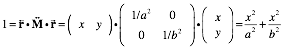
We now introduce a generalization of classical energy-momentum using vector-tensor or matrix notation prevalent in the modern physics. Equations (3.1) thru (3.8) are dressed up in matrix notation starting with P=M·V definitions. Modern physicists use inertia M-tensors to hold mass coefficients M1, M2...etc.
![]() (3.9a)
(3.9a)
Later we will need to upgrade to a full matrix of n2 inertial coefficients Mjk for any dimension n.
![]() (3.9b)
(3.9b)
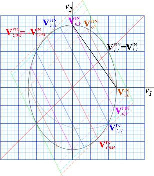
Fig. 3.3 plots
(3.10) below. (Recall Fig. 3.1 plot of (3.1) with 45° diagonal VCOM so: ![]() .)
.)
![]() (3.10)
(3.10)
A product of
total momentum PTotal and ![]() is
expressed by tensor quadratic forms
v•M•u
as follows.
is
expressed by tensor quadratic forms
v•M•u
as follows.
![]() (3.11a)
(3.11a)
It helps to write
this out with the numbers appearing in the original Fig. 3.1 starting with ![]() .
.
![]() (3.11b)
(3.11b)
(3.11) says
momentum PTotal
=250 is the same at IN, FIN, and COM. Now use T-symmetry:![]()
 (3.12a)
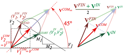
Fig. 3.3 Generic collision geometry. (Recall Fig. 3.1.)
Line-2 of
(3.12a) uses transpose symmetry (Mjk
=Mkj) of the M-matrix so that ![]() .
.
 (3.12b)
In our case (M12 =0=M21) and that implies kinetic energy![]() is the same
at IN and FIN.
is the same
at IN and FIN.
 (3.12c)
However, kinetic
energy ![]() in
Fig. 3.1 is reduced by 1,000 at COM. That is calculated from (3.12c).
in
Fig. 3.1 is reduced by 1,000 at COM. That is calculated from (3.12c).
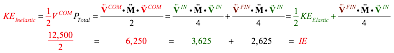 (3.13)
That difference
is inelastic “crunch” energy ![]() or, for
elastic cases, potential energy of compression.
or, for
elastic cases, potential energy of compression.
![]() (3.14)
(3.14)
Potential
energy is given by spatial
tensor quadratic forms such as ![]() detailed
later. Tensors probably get their name from this
application to tension and stress energy.
detailed
later. Tensors probably get their name from this
application to tension and stress energy.
You should note that the less motivated development between (3.1) and (3.5) is improved by a tensor development from (3.11) thru (3.14). The former does not suggest the (3.3)·(3.4) product as easily as the latter suggests the rearrangements going from (3.11) to (3.12) or (3.13). Also arithmetic is displayed clearly and is easier to enter in a computer program involving a full M matrix of any dimension. Finally, (3.12) shows clearly that kinetic energy is conserved if and only if M is transpose-symmetric (Mjk =Mkj).
Tensor forms describe quadratic curves such as ellipses in Fig. 3.1 and the following.
 (3.15)
Geometry
of tensor operator forms is beautiful and powerful for mathematics and physics
as will be shown in later chapters. In quantum theory they define expectation![]() and
transition
and
transition![]() amplitudes.
amplitudes.
Momentum vs. energy (Bang! for the $buck$!): Standard (mks) units
What are momentum P and energy E, really? A flippant answer is Bang! for the $Buck$. We pay a lot of bucks in order to get some bangs in our autos, for example. A less flippant answer based on space-time relativity and quantum wave theory must wait until later. But, we can discuss relations involving P=M·V and E=M·V2/2 and review proper meter-kilogram-second (mks) units to replace haphazard geometrical units used so far. Velocity is V meters per second (m·s-1) and Momentum is P=M·V kilogram meters per second (kg·m·s-1).
Energy is E=M·V2/2 kilogram (meters per second)2 (kg ·m 2·s-2). The E unit is such a mouthful that there is a famous name for it: 1 (kg ·m 2·s-2) = 1 Joule = 1 J.
Our collision analysis did not mention the Force F that SUV or VW feel during their encounters. Force is the rate of being banged in bangs per second, or units of momentum delivered per second, or in (mks), F kilogram meters per second per second (kg·m·s-2). The F unit is another mouthful with a very famous name: 1 (kg ·m ·s-2) = 1 Newton = 1 N. Note: 1 Joule = 1 Newton ·meter = 1 N·m is a common unit of Work, that is, “Force-times-Distance.” Also, 1 Joule per meter = 1 J·m-1 = 1 Newton is a “potential force” unit.
Another important unit is that of power Ð, the rate of $bucks$ paid per second, or in (mks), Ð Joule per second. The famous-name power unit is 1 Watt = 1 Joule per second = 1 J·s -1.
Here is a list of geometric slope and area definitions of important classical mechanical quantities.
Velocity V is slope V =![]() on graph x(t) of position x vs. time t. Position x(t) is area
on graph x(t) of position x vs. time t. Position x(t) is area ![]() of V(t) vs. t.
of V(t) vs. t.
Force F is slope F=![]() on graph P(t) of momentum P vs. time t. Momentum P(t) is area
on graph P(t) of momentum P vs. time t. Momentum P(t) is area ![]() of F(t) vs. t.
of F(t) vs. t.
Force F is slope F=![]() on graph E(x) of energy E vs.
position x. Energy E(x) is area
on graph E(x) of energy E vs.
position x. Energy E(x) is area ![]() of F(x) vs. x.
of F(x) vs. x.
Power Ð is slope Ð =![]() on graph E(t) of energy E vs. time t. Energy E(t) is area
on graph E(t) of energy E vs. time t. Energy E(t) is area ![]() of
of ![]() vs. t.
vs. t.
These and other relations (in calculus form) are collected below in preparation for discussion later on.
Quick review of kinetic relations and formulas
The suffix kinetic refers to energy connected directly to velocity of motion (“kinos” means moving). Kinetic energy KE is distinct from potential energy (PE is “stored” energy) or entropic energy (entropy is chaotic or “trashed” energy like heat) that is reviewed later in Ch. 6 and Ch. 7.
We now give a quick algebraic run-down of energy-related formulas to be introduced with more detail and geometry in Ch. 7. (See (7.5a) to (7.5d) in particular.) Readers with calculus or physics knowledge may use this to review to connect our geometrical developments with the more conventional ones.
Relations of energy W and space x
Energy or work may be defined by a delta-work product ÄW=F·Äx of
force F
and distance-Äx-pushed. More precisely, W is an
integral ![]() ,
the area of a Fvs.x
work-plot. Power,
a time rate
,
the area of a Fvs.x
work-plot. Power,
a time rate![]() of energy
production, is the product
Ð=F·V of force and velocity
of energy
production, is the product
Ð=F·V of force and velocity![]() . So,
. So, ![]() or
or ![]() .
.
Relations of momentum P and time t
Momentum may be defined by a delta-momentum
product ÄP=F·Ät of force F and time interval Ät. More precisely, P is an
integral ![]() ,
the area of a Fvs.t
plot. Force,
a time rate
,
the area of a Fvs.t
plot. Force,
a time rate![]() of momentum production, is a product F=M·a
of mass and acceleration
of momentum production, is a product F=M·a
of mass and acceleration![]() . (F=M·a is
called Newton’s
“2nd Law.”)
. (F=M·a is
called Newton’s
“2nd Law.”)
With ![]() , energy
integral
, energy
integral ![]() is
is
![]() ,
the area under a
V vs.P plot where P=M·V
is momentum. For a single mass M
this area is kinetic energy:
,
the area under a
V vs.P plot where P=M·V
is momentum. For a single mass M
this area is kinetic energy: ![]() M·V2.
M·V2.
Table 3.1 of kinetic relations
![]()
![]()
![]()


(3.16a) (3.16b) (3.16c) (3.16d)
Exercise 1.3.1
Plot a (VSUV-1,VSUV-2)=(60,10) collision like Fig. 3.1 but with an identical M=4 SUV replacing the VW.
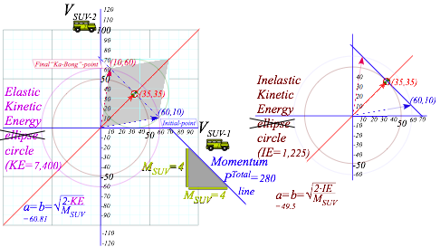
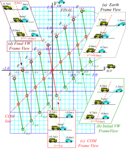
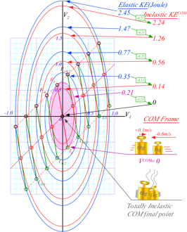
Fig. 3.4 Galilean Frame Views of collision like Fig. 2.5 or Fig. 3.1 with Bush SUV. (a) Earth frame view
(b) Initial VW frame (VW initially fixed) (c) COM frame view (d) Final VW frame (VW ends up fixed)
Fig. 3.5 Momentum (P=const.)-lines and energy (KE=const.)-ellipses appropriate for Fig. 3.4.
Exercise
1.3.2. Ch. 1-5 contains
geometric description of 1D-2-body collisions. Most examples originate from
initial velocity vectors ![]() for
which m1 and m2
have equal speeds (in this case unit speed).
for
which m1 and m2
have equal speeds (in this case unit speed).
This exercise is intended to help match algebra and geometry by asking for the simplest formulas for the various velocities in a figure above that are final elastic results of the following initial velocity vectors.
a. ![]() b.
b.
![]() c.
c.
![]() d.
d.
![]()
Derive the IN
and FIN components of all vectors in terms of masses m1 and m2
only assuming the same total KE as ![]() has. (Check
your results against figure in which ratio 2=m1/m2 holds.)
has. (Check
your results against figure in which ratio 2=m1/m2 holds.)
Indicate where the time reversed vector T·VIN of each VIN lies.
Give a formula for the orange (dashed) and green (solid) tangent line slopes in terms of m1 and m2.
…and compare to slope of the black line connecting major and minor radii in terms of m1 and m2.
Exercise 1.3.3. Quick construction of Energy ellipses
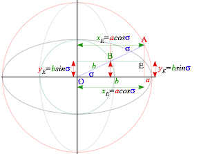
Graph paper facilitates construction of energy ellipses given the two radii a and b in (3.7). The first step is to draw concentric circles of radius a and b. Then any radial line OBA “points” to a point E on the ellipse.
Ellipse point E lies at the intersection of a vertical line AE thru radial intersection A with circle a and a horizontal line BE thru radial intersection B with circle b.
Graph grid “finds” E for a radius OBA, no need to draw AE or BE. You can pick x and find y or vice-versa.
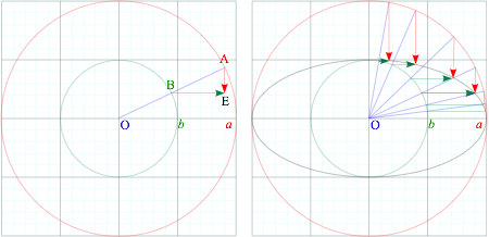
Exercise Fig. 3.6 Ellipse construction
Ellipse coordinates (xE=a·cos ó, yE=b·sin ó) are rescaled base and altitude (xr=r·cos ó, yr=r·sin ó) of Fig. 1.4.
Exercise Fig. 3.7 Complimentary analytic ellipse geometry
Verify that the values (x =a·cos ó, y =b·sin ó) satisfy an ellipse equation (3.7b).
A dual or complimentary (gray) ellipse results if compliment angle óc=ð/2−ó is used so x and y values switch.
Chapter 4. Dynamics and geometry of successive collisions
Mechanics gets difficult for many collisions, dimensions, or masses. A single one-dimensional two-mass (1D-2-body) collision occupies Ch. 2-3. Now we do more dangerous things such as an X2-super bouncer from Project Ball, a 1969 class project. (Am. J. Phys. 39, 656 (1971)) See product liability disclaimer in Fig. 4.1.
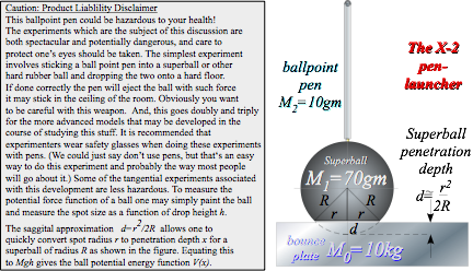
Fig. 4.1 The X2-pen launcher with product liability disclaimer.
At
first, the X2 looks like a 1D-2-body device. A superball(©™Whammo Corp.) of mass M1
=70gm launches a ballpoint pen of mass M2 =10gm. But, it has a 3rd body,
bounce plate mass-MO=10kg shown by a rectangle in Fig. 4.1.
Actually the third body most responsible for this experiment is good old Mother
Earth of mass![]() .
(Earth mass
.
(Earth mass![]() and solar mass
and solar mass![]() are good-to-2-figure numbers for astrophysicists to remember. More precisely:
are good-to-2-figure numbers for astrophysicists to remember. More precisely: ![]() and
and ![]() .)
.)
Collisions of very large with very small masses beg thorny questions (Like, “What IS mass?” or how do we deal with it?) As a mass ratio M1/ M2 approaches zero or infinity the slope of the P-conservation line in (V1,V2)-space (Recall Fig. 3.2.) approaches infinity or zero, respectively, as drawn in Fig. 4.2(a-b).
Geometric construction in Fig. 4.2a of final velocity for an elastic collision is a vertical reflection thru the COM point (V1=V2) on the P-line if M1>> M2 or else a horizontal reflection in Fig. 4.2b if M1<< M2. Inelastic final points approach the COM point more closely if inelasticity is significant. (Recall Fig. 3.2.)
You
should understand how a relatively large mass may give huge momentum to a
smaller one but transfer only tiny amounts of energy. Each P-line in Fig. 4.2 is part of a KE-ellipse. In the COM frame (where the COM point is at origin) the P-line sits on top of an entire E-ellipse as the ratio M1/
M2 approaches (a) infinity or (b) zero. I visualize COM P-lines as ultra-thin ellipses between I0 and F0
and other P-lines in Fig. 4.2 as segments of a
KE-ellipse that has (a) a huge V2-axis
![]() or
(b) a huge V1-axis
or
(b) a huge V1-axis
![]() .
.
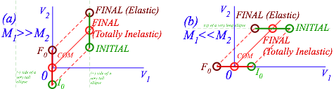
Fig. 4.2 Extreme mass-ratio collisions (a) M1/ M2 approaches infinity. (b) M1/ M2 approaches zero.
Fig.
4.2a reflects our common experience of a bouncy ball of mass M2 hitting the Earth of mass ![]() with velocity –V0(point I0) and being reflected with velocity +V0(point F0). While standing in the Earth frame, one
is very nearly in the COM frame, too. Earth’s COM velocity is a tiny fraction
with velocity –V0(point I0) and being reflected with velocity +V0(point F0). While standing in the Earth frame, one
is very nearly in the COM frame, too. Earth’s COM velocity is a tiny fraction ![]() of the
apparent ball velocity V0. For super-balls of mass M2=60gm, the fraction
of the
apparent ball velocity V0. For super-balls of mass M2=60gm, the fraction ![]() is 0.06/(6·1024)=10-26.
is 0.06/(6·1024)=10-26.
Bounce momentum absorbed by Earth is 2 M2V0 (or M2V0 if the ball goes “Ka-runch!”) but Earth absorbs at most a tiny KE of ![]() , that is, a
fraction 10-26 of ball KE:
, that is, a
fraction 10-26 of ball KE: ![]() . Moreover,
for elastic collisions, Mother Earth returns all
the KE to M2 but she absorbs double momentum P=2 M2V0.
. Moreover,
for elastic collisions, Mother Earth returns all
the KE to M2 but she absorbs double momentum P=2 M2V0.
However, common experience does not prepare us for X2 easily rebounding M2 with more than twice its drop velocity in Fig. 4.3. (As we’ll see that means M2 rises to more than four times its drop height!)
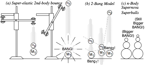
Fig. 4.3 n-Body collision experiments. (a) X-2 drop. (b) Independent collision model. (c) Ball towers.
Independent collision models (ICM)
To
compute final velocities of M1 and M2
it helps to idealize the collision of three bodies M1, M2, and ![]() as a sequence
of two separate 2-body collisions that are completely determined by P and KE conservation. First M1 bounces off Earth
as a sequence
of two separate 2-body collisions that are completely determined by P and KE conservation. First M1 bounces off Earth![]() . Only then
does M1 knock M2
to a faster speed as in Fig. 4.3b. The first collision is labeled Bang-1(01) in Fig. 4.4a followed by Bang-2(12) in Fig. 4.4b. The first Bang-1(01) between Earth
. Only then
does M1 knock M2
to a faster speed as in Fig. 4.3b. The first collision is labeled Bang-1(01) in Fig. 4.4a followed by Bang-2(12) in Fig. 4.4b. The first Bang-1(01) between Earth![]() and M1 has a horizontal line like the I0F0 line in Fig. 4.2b. The second Bang-2(12) between mass M1 and M2
has a line of slope -M1/
M2 =-7 for a M1 =70gm and M2
=10gm (that of a superball and pen,
respectively). The
Bang-2(12) line
is like the IF line in Fig. 3.1 or Fig. 3.2.
and M1 has a horizontal line like the I0F0 line in Fig. 4.2b. The second Bang-2(12) between mass M1 and M2
has a line of slope -M1/
M2 =-7 for a M1 =70gm and M2
=10gm (that of a superball and pen,
respectively). The
Bang-2(12) line
is like the IF line in Fig. 3.1 or Fig. 3.2.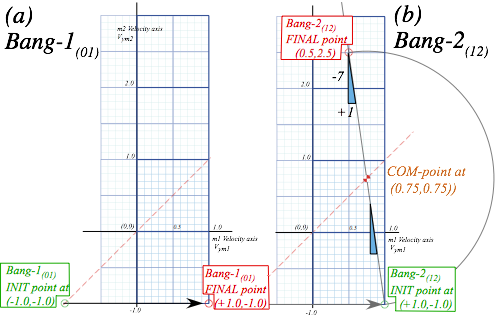
Fig. 4.4 (V1-V2)-plot of 2-Bang collision. (a) M1 bounces off floor. (b) M1 hits M2 head-on.
This
approximation is called an independent collision model
(ICM) and is one secret to analyzing such
1D-3-body bang-up that otherwise has too many unknown velocities to be found by
just two equations ÄP=0 and ÄKE=0 alone. ICM is exactly true if we
initially separate M1 and
M2 so three M1, M2, and ![]() never collectively bargain for available momentum and
energy. ICM also applies to n-ball towers in Fig. 4.3c. They give very
high-energy ejections and serve as classical models for supernovae. (N-body bangs are in Ch.8.)
never collectively bargain for available momentum and
energy. ICM also applies to n-ball towers in Fig. 4.3c. They give very
high-energy ejections and serve as classical models for supernovae. (N-body bangs are in Ch.8.)
Velocity geometry suggests a family of X2 solutions as shown in Fig. 4.5 for a range of mass ratio M1/M2. This is an advantage of geometric solutions. Just a few points in Fig. 4.5a show all elastic (V1-V2) points lie on the 45°-line CPL. Extreme or optimal cases are located in Fig. 4.5b.
First, the upper limit for elastic final
velocity is V2=3·V0 at pt-I
for infinite mass ratio M1/M2![]() . If no energy is lost, a particle of
dust on a superball could be ejected three times the speed that the ball hits
the floor. (And, it could go nine (9=32) times the drop height. However, the
elastic ICM model is not so good for tiny M2 due to weak molecular forces. So
bouncing balls don’t embed dust in ceilings. (But in a vacuum...!)
. If no energy is lost, a particle of
dust on a superball could be ejected three times the speed that the ball hits
the floor. (And, it could go nine (9=32) times the drop height. However, the
elastic ICM model is not so good for tiny M2 due to weak molecular forces. So
bouncing balls don’t embed dust in ceilings. (But in a vacuum...!)
Second, an optimal performance case is shown by pt-M where the collision achieves a 100% transfer of energy to projectile M2. The M-point is the intersection of the CPL line with the V2-axis on which the M1-ball velocity is zero. (V1=0) There mass ratio is M1/M2=3.0, the slope of the M-line.
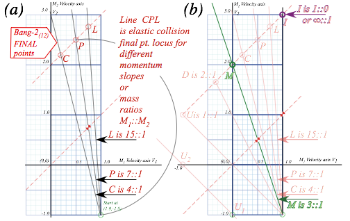
Fig. 4.5 X2-Final (V1,V2) (a) Final point locus. (b) Infinite ratio pt. I and maximum transfer pt. M.
Another singular point U is for unit ratio M1/M2=1, a familiar ratio for players of billiards or pool. U undergoes inversion of velocities (+1,-1)-> (-1,+1). (Its COM point lies at origin.) If the U-line is boosted by (-1) to (0,-2)-> (-2,0) it is like a straight elastic pool shot. A 100% of KE transfers from a moving ball to an equal sized ball that was stationary. The same process at half that speed is (0,-1)-> (-1,0) shown by the Galileo-shifted line U1-> U2 in the lower left hand side of Fig. 4.5b.
Points D between U and M have ball M1 knocked to negative velocity by the down-coming M2. Then M1 hits the floor (Earth) at velocity –v to rebound at +v. For unit ratio case U, M1 and M2 rebound quite like a rigid body. Below U, ball M1 rebounds at a speed faster than M2 to hit M2 again. In cases of low mass ratio, (M1/M2<<1) mass M1 must hit M2 many times to turn it around. We will study this effect shortly.
Integrating velocity plots to find position
It is important to see how velocity values of Fig. 4.4b are turned into space-time position plot lines. Consider the first collision (Bang-1(10)) in Fig. 4.6a and corresponding space-time paths in Fig. 4.6b. Initial velocity Vy1(0)=-1.0 gives a slope (distance)/(time) of an M1 path but doesn’t tell where is the path or particle. The same for velocity Vy2(0)=-1 of M2 in Fig. 4.6a. The paths need location, location,…
Initial position values such as (y1(0)=1, y2(0)=3) locate the paths as shown in Fig. 4.6b. Each path keeps its slope until a collision (Bang-1(10)) between M1 and the floor occurs at y1(t=1) where its path and the floor intersect. Then, according to Fig. 4.6a, M1 bounces its slope from Vy1=-1 up to Vy1=+1. Meanwhile, the upper path (M2) maintains its down slope of Vy2=-1 until it intersects the rising path of M1.
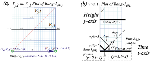
Fig. 4.6 Plots of 1st collision (Bang-1(10)). (a) Velocity-velocity plot. (b) Space-time plot.
At time (t=2) there is an intersection of paths and the 2nd collision (Bang-2(12)) between M1 and M2 at space-time point (y1(2)=1, y2(2)=3). This gives Vy1=0.5 and Vy2=2.5 in Fig. 4.4b or in Fig. 4.7a-b below. Then to keep M2 from flying away we install an elastic ceiling at y=7.
The
game becomes more interesting as Bang-3(20) between the ceiling (part of Earth ![]() ) is shown in
Fig. 4.7b by a vertical arrow (like an IF
line in Fig. 4.2a) reflecting
M2 to speed Vy2=-2.5. Then M2
has Bang-4(12) between M1
and itself that sends it back to the ceiling at a blistering speed of Vy2=+2.7 as M1
returns more slowly toward the floor with velocity Vy1=-0.5.
) is shown in
Fig. 4.7b by a vertical arrow (like an IF
line in Fig. 4.2a) reflecting
M2 to speed Vy2=-2.5. Then M2
has Bang-4(12) between M1
and itself that sends it back to the ceiling at a blistering speed of Vy2=+2.7 as M1
returns more slowly toward the floor with velocity Vy1=-0.5.
The high speed of M2 lets it go to the ceiling for Bang-5(20) and return to knock M1 down once more (Bang-6(12)) before M1 hits the floor at Vy1=-0.9. (Bang-7(10)) Then M2 having lost speed to Vy2=+1.5 hits the ceiling (Bang-8(02)) and returns for Bang-9(12) with M1 rising at Vy1=+0.9.
Masses are treated as point-masses moving
along straight lines between collisions in space-time plots. This is an ideal
gravity-free ICM approximation with only straight lines in VV-plots. So we may derive motion without having to integrate
the kinetic equations at the end of Ch. 3.
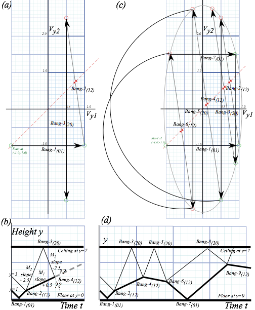
Fig. 4.7 Collision sequence. (a-b) Up to Bang-4(12). (c-d) Up to Bang-9(12).
For comparison, a force-law simulation using BounceIt of the bang sequence of Fig. 4.7 is shown in Fig. 4.8. It has finite radius balls instead of ideal point particles, yet compares quite well. (So far as it goes.)
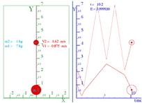
Fig. 4.8 BounceIt x-vs.-t simulation to compare with Fig. 1.4.7d up to Bang-6. (V1/V2 =7/1.)
Fig. 4.7c and BounceIt V1-V2 simulations in Fig. 4.9 build an ellipse out of multiple IF lines. (This is a quite non-traditional ellipse construction!) Ellipse radii (a,b) follow from KE conservation equation (3.7b).
As time increases (Fig. 4.9a to Fig. 4.9c) the ellipse may fill with IF-lines that are dense (ergodic) or else just retrace sets of paths as in Fig. 4.9b. (Ch. 5 treats non-ergodic paths.) High sensitivity-to-initial-conditions-or-parameters (STICOP) means tiny ICOP variation has big effects. Extreme STICOP gives stochasticity or chaos.
Vector notation and space-space plots
Balance equation (3.4) concisely sums up preceding constructions or plots of elastic collisions.
 or:
or:![]() (3.4)repeated
(3.4)repeated
More concise notation uses vector equations or arrays.
 (4.1)
(4.1)
It saves writing two (=)’s and two (-)’s. Also, each column vector may be labeled by a “fat” letter.
![]() (4.2)
(4.2)
The Gibbs
vector form of equation
(3.4) or (4.1) uses fat-v and/or over-arrow-![]() .
.
vFIN
= 2 VCOM – vIN
, or:
![]() . (4.3)
. (4.3)
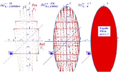
Fig. 4.9 BounceIt V1-V2 simulation up to (a) Bang-15 (b) Bang-150 and (c) beyond.
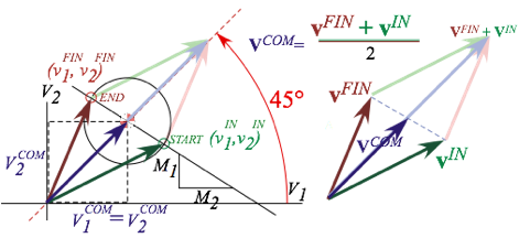
Fig. 4.10 Vector collision velocity diagrams (After equation (4.3) and virtually identical to Fig. 3.3.)
Note vector VCOM bisecting the (vIN+ vFIN)-parallelogram diagonal as per T-symmetry relation from (3.12a) and Fig. 3.3. Here vectors v=(v1, v2) denote two particles each in one-dimension. More common is vector v=(vx, vy) (or v=(vx, vy, vz)) for one particle in two-dimensions (or three dimensions).
Fig. 4.11 shows how velocity v(n) vectors find results of Bang-1(01) and Bang-2(12) collisions in Fig. 4.7. What’s new is a space-space y2 vs. y1 or position-vector y(n)-plot whose paths are spatial-trajectories or just plain trajectories. Space-time paths are found in Fig. 4.6 and Fig. 4.7 by transferring velocity slopes over to the space-space or space-time plot, but vectors in Fig. 4.11 simplify this process. Again, ideally small masses called point masses are assumed.
As the construction steps in Fig. 4.11 show, one easily transfers each velocity vector v(n) from the V2 vs.V1 plot so it points away from start point y(n) in the y2 vs. y1 plot. Step-0 does this by drawing initial velocity v(0)=(-1,-1) to point away from our given initial position y(0)=(1,3). Then you extend that v-vector until it hits the floor (as v(0) does at y(1)=(0,2)), or else hits the collision line (y2=y1) (as v(1) does at y(2)=(1,1)), or else hits the ceiling (as v(2) does at y(3)=(2.2,7).). Each such “hit” is a Bang, Bang-1(01) at y(1), Bang-2(12) at y(2), or Bang-3(20) at y(3). Then from each Bang-n position point y(n) is drawn the next v(n)-velocity vector from the V2 vs.V1 plots. This process continues in exercises that lead to Fig. 4.12 and beyond.
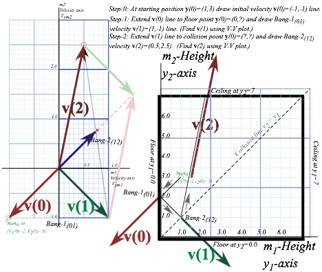
Fig. 4.11 Vector collision velocity diagrams with Velocity-Velocity space and space-space.
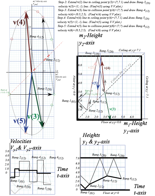
Fig. 4.12 Vector collision diagrams continued with velocity-time and space-time plots added.
Help! I’m trapped in a triangle.
The trajectory in these figures is confined to the triangle above the 45°-collision line. Our model keeps m2 above m1. The right-hand “ceiling” in the figures never is hit because m1 always is knocked down by m2 before it touches the ceiling, and m2 never sees the floor because m1 is in the way. (Modern physicists beware! Quantum theory doesn’t encourage this feature. Quantum objects pass easily through each other! )
Two balls in 1D vs. one ball in 2D
For ball-Earth collisions involving ceiling or floor, the paths bounce in the space-space plot as though they’re inside a box. Only one component V1 or V2 changes each time and only by changing ±sign. Off the floor: (V1 ,V2) changes to (-V1,V2) , off of ceiling: (V1,V2) changes to (V1,-V2). It is like a single particle bouncing around a pool table. Here (V1,V2) acts like (VX ,VY) in two dimensions, so two particles in one-dimension use graphs similar to one particle in two dimensions, an interesting analogy in quantum theory.
Angle of incidence=Angle of reflection (or NOT)
When paths bounce off the floor and ceiling in the space-space plot, the angle of incidence equals the angle of reflection just as light rays reflect off mirrors. (Newton imagined little light corpuscles bouncing around.) It is customary to measure path angles from the normal or perpendicular to a mirror so a normal bisects the angle between the incident and reflected paths.
For m1-m2 Bangs off the 45°-collision
line, the bisecting line has the slope -M1/M2=-7. It is like having mirror facets at
slope M2/M1=1/7 along the 45°-collision
line. For equal-mass-(M1=M=M2) balls, or one
ball in two dimensions, the bisecting line slope at
the 45°-collision line is –1 or -45° and the collision line acts like a
unit-slope mirror on a triangular billiard table. It is not quite that simple
if![]() .
.
Consider the two collisions Bang-3(20) and Bang-4(12) in Fig. 4.12. Velocity v(2) bounces off the ceiling in Bang-3(20) into v(3), whose velocity slope is close to the mass-ratio M1/M2 which is 7:1 here. So the next collision Bang-4(12) bounces v(3) off the diagonal into v(4) which is close to –v(3). It’s followed by another ceiling bounce Bang-5(20) into v(5) heading down for another collision Bang-6(12).
Lower Fig. 4.12 has a velocity vs. time plot next to a space-time plot. (A y-t plot in gray is under the V-t plot, too.) Each Bang means a change in velocity for any particle involved in the collision. By Newton’s 2nd law (3.10c) each change in velocity, v to v+Äv, or better, each change in momentum, mv to m(v+Äv), requires a force impulse F·Ät= m(Äv) on each mass that changes. Shortly, we study ways to deal with this F.
The velocity-velocity (v1,v2) plots, such as the left side of Fig. 4.12, fall in a category known as kinematics, or momentum analysis, which is concerned with how things are going, where they’re headed, or what is their velocity or momentum and energy. (kinos means movement.)
In contrast, the space-time plots, such as the right side of Fig. 4.12, fall in a category known as dynamics, or coordinate analysis, which is concerned with how things are located, where they are, or what are their coordinate or position and time schedules. (dynos means change.) We introduced the space-space (x1,x2) plot, another geometric or trajectory representation of dynamics.
Before going on, let’s compare how kinos and dynos play out in classical Newtonian physics versus their corresponding roles in quantum physics. This is a preview for later Unit 4, Unit 7, and Unit 8.
Dynos and Kinos: Classical vs. quantum theory
In Newtonian physics, a precise position plot (yk vs. time) lets you find a precise velocity plot, too, and, a velocity plot (Vk vs. time) lets you find a position plot if you know starting position values. (We did just that in Fig. 4.7 and Fig. 4.11.) In calculus, finding position from velocity values is called integration, and finding velocity from position values is called differentiation. Of the two, the latter is formally easier but numerically and experimentally more sensitive to imprecision and noise.
In quantum physics, having a precise velocity plot renders a position plot meaningless and vice-versa! Werner Heisenberg was the first to state this quantum idea, now known as Heisenberg’s Principle. If you know momentum exactly, that means a uniform wave is everywhere, and all positions are equally possible. If you know position exactly, that means every momentum is possible, implying a “wave-bomb” about to blow up the universe! (Neither of these extremes really exist and fortunately so for the last one.)
All this sounds crazy to most of us who are born-and-bred Aristotelean-to-Newtonian students. It is difficult enough to go from Aristotle’s what-you-see-is-what-you-get (WYSIWYG) universe to Newton’s corpuscular one. A quantum universe is yet another step removed on the WYSIWYG scale.
A way to see the quantum universe (Perhaps, it is the way.) is to learn about wave kinematics and dynamics without Newtonian corpuscles and see how waves mimic corpuscles and do so quite cleverly. The quantum universe is a WYDAWYG (waves-you-don’t see-are-what-you-get) world!
So our plan is to cast classical Newtonian kinematics and dynamics in a form that carries over into vibration and wave kinematics and dynamics. It is done by analogy with classical waves such as sound waves, water waves, and (most important) light waves. Many classical wave analyses invoke corpuscles (including, for Newton, light waves) so these analogies, like any analogy, need critical use of an Occam’s razor that must be sharpened. Above all, symmetry (and same-try) principles must be taken seriously.
IF-ellipse geometry of Ch. 3 relates velocity, momentum and energy, and Ch. 4 derives space-time paths. Later this relates Lagrangian and Hamiltonian mechanics and finally leads to geometries of relativity and quantum mechanics. Then space-space and space-time plots relate to modern physics in subtle ways.
Exercise 1.4.1: Construct a history of a 4:1 mass ratio bounce. x1(0)=1.5, x2(0)=3.0, v1(0)=-1, v2(0)=-1
Ceiling height=7.0.(For bottom row: Ceiling height=6.0 ) The 4:1 mass ratio case is surprisingly periodic.
Exercise 1.4.2: Complete Fig. 4.7 and Fig. 4.11 by constructing more steps using same ceiling height=7.0.
Continue until you reach the “gameover” point of last possible M1-M2 collision assuming the floor is open after Bang-1 so both masses fall thru indefinitely. When and where do they last collide?
Note, position y(n)-vectors of the Bang-n points are not drawn in Fig. 4.12 to avoid clutter.
Chapter 5 Multiple collisions and operator analysis
Analysis of many collisions with very different masses requires an advanced kind of geometry and algebra involving matrices and symmetry operators. Similar analysis is needed for quantum theory so this is a good opportunity to learn about these concepts using a more “down-to-Earth” classical bang physics.
Doing collisions with matrix products
Fig. 5.1 shows a big mass m2=49 bang a little mass m2=1 more than ten times off the ceiling
before being halted. This tests our collision precision! To check our results
we use our previous vector equation (4.1) to make a matrix equation in (5.1) with ![]() and
total mass M = m1+ m2.
and
total mass M = m1+ m2.
![]() (4.1)repeated
(4.1)repeated 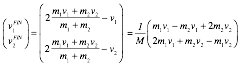 (5.1a)
(Let ![]() and
and![]() here.) Vector
equation (5.1a) is converted to matrix equation
here.) Vector
equation (5.1a) is converted to matrix equation ![]() in (5.1b).
in (5.1b).
![]() (5.1b)
(5.1b)
Each IN-to-FIN bang is a ![]() operation
(5.2a). Matrix product
operation
(5.2a). Matrix product ![]() (5.4b)
is bang-M following bang-N.
(5.4b)
is bang-M following bang-N.
![]() (5.2a)
(5.2a) ![]() (5.2b)
(5.2b)
Matrix M
operates column-by-column on another matrix N
as it does on a vector v. The
off-the-ceiling matrix C =![]() changes (v1, v2) to (v1, -v2) (Odd-n Bang-n(02)) A 2-ball collision matrix M (Even-n Bang-n(12)) and ceiling bang C
act p-times in matrix products
changes (v1, v2) to (v1, -v2) (Odd-n Bang-n(02)) A 2-ball collision matrix M (Even-n Bang-n(12)) and ceiling bang C
act p-times in matrix products ![]() to give Fig. 5.1.
to give Fig. 5.1.
![]() (5.3)
(5.3)
(5.4) shows (p=5) double-bangs ![]() following a floor-bounce
following a floor-bounce ![]() or 11 bangs in all.
or 11 bangs in all.
 (5.4)
(5.4)
![]()
Even after 9 bangs, big m1 still has a small upward velocity v1=0.2925.
After Bang-11(02) big m1 is nearly stopped and little m2 is coming down at v2=-7.071 with all the energy!
![]() (5.5)
(5.5)
Look out below! As m1 turns back it crosses v1=0 axis in Fig. 5.1a. The greatest curvature (acceleration and force) for the path of m1 is between Bang-8 and Bang-14 in Fig. 5.1b just when m2 is busiest.
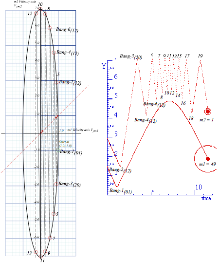
Fig. 5.1 Multiple Bangs of the m1=49 and m2=1 superball system. (a) V vs V plot. (b) Y vs time.
Big m1 is repelled down by repeated m2 hits and gains speed as m2 loses it. If no floor intervenes to rebound m1 there comes a final bang that leaves m2 slower than m1 who falls away so m2 can’t hit it again. (We’ll call this a game-over point. As an exercise, you will be asked find it for various cases.)
However, if a floor intervenes, then a 2nd
floor-bounce matrix F=![]() changes (v1, v2) to (-v1, v2) and bounces ball-m1 back up to start the whole process over
again. Ball-m1 does another graceful up-then-down time
trajectory very much like the one shown on the right-hand side of Fig. 5.1.
changes (v1, v2) to (-v1, v2) and bounces ball-m1 back up to start the whole process over
again. Ball-m1 does another graceful up-then-down time
trajectory very much like the one shown on the right-hand side of Fig. 5.1.
Except for floor bounces, the m1-ball in Fig. 5.1 experiences a smoother flight than in Fig. 4.7 where a more massive m2-ball jerks it severely. A smaller mass m2 has less momentum-per-bang and gives a quasi-continuous force field for m1. We will derive a funny kind of force and potential field theory from this.
Rotating in velocity space: Ticking around the clock
Here is an example of geometry and slope ratios being helpful. If you view the ellipse in Fig. 5.1a lower-edge-on (and do the exercise to finish it!) you may see it as a circular clock with each double-bang (odd-bangs 1,3,5,…) rotating the v-vector like a clock hand ticking equal-angle jumps around a dial.
You can make an energy ellipse (2E=m1v12+ m2v22) like Fig. 5.1(a) sketched in Fig. 5.2(a) into an energy circle (2E =V12+V22) like Fig. 5.2(b) by rescaling velocity (v1, v2) to (V1 = v1·√m1, V2 = v2·√m2).
V1=v1·√m1, V2=v2·√m2 where: 2E=m1v12+ m2v22=V12+V22 (5.6)
Big-V variables replace little-v’s by setting (v1 =V1/√m1, v2 =V2/√m2) in matrix relation (5.1).
![]() (5.1)repeated
(5.1)repeated ![]() (5.7)
(5.7)
Clearing scale factors √mk gives the following big-V matrix relations to replace (5.1) above.
![]() (5.8)
(5.8) ![]() (5.9)
(5.9)
The trick is to notice a Pythagorean relation x2+y2=1 for the circular bang-matrix components.
![]() (5.10a)
(5.10a)
The matrix can be defined using sinè and cosè shown for m1=49 and m2=1 and angle è =16.26° in Fig. 5.2(c).
![]() (5.10b)
A 1-Bang matrix is a reflection by è. Our 2-Bang
matrix is a rotation by
angle -è =-16.26° in V space.
(5.10b)
A 1-Bang matrix is a reflection by è. Our 2-Bang
matrix is a rotation by
angle -è =-16.26° in V space.
![]() (5.11)
(5.11) ![]() (5.12)
(5.12)
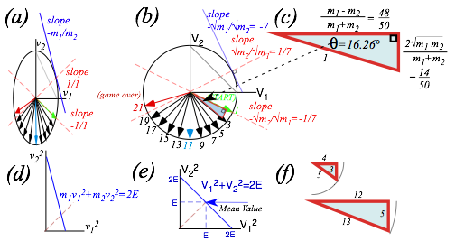
Fig. 5.2 Velocity-velocity clocks. (a) Energy ellipse (As in Fig. 5.1) (b-c) Energy bang-clock angles
(d) Velocity-squared E-plot. (e) Mass-scaled V-squared E-plot. (f) Integral right triangles
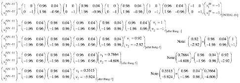
Matrix (5.12) reduces N-double-bang chains like (5.4). N products of matrix (5.9) are done if è =16.26° in (5.12) is replaced by Nè =81.30° to give (5.13) below. (We take N=5 double-bangs to check against (5.5).)
![]() (5.13a)
(5.13a)
Relate V’s to v’s by (V1=v1√m1, V2=v2√m2) gives (5.5). Note ![]() follows initial floor F: (v1, v2)=(1,-1).
follows initial floor F: (v1, v2)=(1,-1).
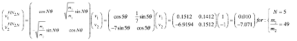 (5.13b)
Without a 2nd floor-bounce-back operation F, this sequence ends near bang-21 our “game-over” point. (See exercise 5.1.) Matrix group products clarify collision sequences so they may be “engineered.”
Statistical mechanics: Average energy
If two balls of mass m2=1 and m1=7 bounce back and forth between wall the small ball goes faster on the average than the bigger one. How much faster? Let’s assume that arrows on the scaled velocity clock in Fig. 5.2(b) get uniformly distributed around its circle after many collisions. (Fig. 5.2(b) shows only m1-m2-bounce arrows. m2-ceiling-bounce-arrows fill up the upper half.) A ball’s velocity and momentum must sum and average to zero otherwise it will not stay in the region between the floor and the ceiling.
But, what is average squared-velocity v2 of each ball? An energy plot in the space (V1)2 vs (V2)2 of scaled velocity-squared helps to answer this. The result is a 45° line shown in Fig. 5.2(e). In other words points on the circle in Fig. 5.2(b) get mapped onto the 45° line in Fig. 5.2(e) by KE conservation.
(V1)2 + (V2)2 = 2 KE = m1(v1)2 + m2(v2)2
The average of all points on the 45° line is its bisector.
(V1)2 = KE = (V2)2 or: m1(v1)2 = KE = m2(v2)2
This gives the average velocities or root-mean-square-speeds v1rms and v1rms of m1 and m2.
![]()
![]() (5.14)
(5.14)
Each ball, regardless of mass, gets equal share (50% if there are just two) of the total energy. So, if m1 is 7 times m2 then the mean speed of m2 is √7=2.65 times faster than that of m1. The 1st bang in Fig. 4.4 gives 2.5.
Bonus: Rational right triangles
Geometry often offers interesting numerics. In this case, the general right triangle in Fig. 5.2(c) makes integer or rational fraction solutions to the Pythagorean sum a2+b2=c2 such as the famous (a=3,b=4,c=5) right triangle. Perfect-square mass values (m1 and m2=1, 4, 9, 16, 25, 36, 49, 81, 100,…) will give integral valued right triangle altitude a=√(4 m1·m2), base m1-m2, and hypotenuse m1+m2. Examples in Fig. 5.2 are (a=14,b=48,c=50) for (m1=49, m2=1) and (a=12,b=5,c=13) for (m1=9, m2=4).
Reflections about rotations: It’s all done with mirrors
In
1843 Hamilton discovered his quaternion algebra
{1,i,j,k}, a mathematical jewel. In 1930 Pauli
found related spinor matrices {1,óX, óY, óZ}. We label Pauli matrix óZ as sigma-A=óA (A
for Asymmetric) and óX as sigma-B=óB (B
for Balanced). They are
Hamilton’s k
and i with an
imaginary factor ![]() attached.
attached.
![]() (5.15a)
(5.15a) ![]() (5.15b)
(5.15b)
Other matrices, sigma-C=óC (C for Circular) and sigma-0=ó0(0 for “Origin”) are products like óAóB or óA2.
![]() (5.15c)
(5.15c) ![]() (5.15d)
(5.15d)
Hamilton’s
{i,j,k} square to -1. (i2=j2=k2=-1) That is like ![]() . But, Pauli-ó’s square to +1. (1=óX2=óY2=óZ2.)
. But, Pauli-ó’s square to +1. (1=óX2=óY2=óZ2.)
We now relate ó-matrices to simple super-ball collision reflections and rotations shown in Fig. 5.2. For example, the óA is our “ceiling bounce” C in (5.3) and our “floor bounce” F in (5.3) is just - óA.
![]() = C (5.15a)
= C (5.15a) ![]() = F (5.15b)
= F (5.15b)
A geometric view of óA (or - óA) is mirror reflection thru Cartesian x (or y) axes in Fig. 5.3a while óB (or - óB) is reflection thru mirror planes tilted at angle ð/4 (or −ð/4) between x-y axes in Fig. 5.3b. General reflection óö thru a mirror plane tilted at angle ö/2 (Fig. 5.3c) is a sum (5.15c) of óA cosö and óB sinö. We now verify this.
![]() (5.15c)
(5.15c)
Like
all reflections, óö
must square-to-one. (óö2=1) It does so because óA2=1=óB2 and óAóB
=-óBóA. We test óö on unit vectors![]() and
and ![]() and see
that matrix algebra checks with geometry in Fig.5.3c.
and see
that matrix algebra checks with geometry in Fig.5.3c.
![]() (5.16a)
(5.16a) ![]() (5.16b)
(5.16b)
Geometry Fig. 5.3d also shows that a product ó2ó1 of any two reflection matrices is a rotation matrix R.
In Fig. 5.3d óöóA is right-hand rotation R+ö but óAóö=R−ö in Fig. 5.3e is left-handed. Rotation angle ö is twice the angle ö/2 between mirrors. Direction of rotation ó2ó1 is from 1st mirror (of ó1) to 2nd mirror (of ó2).
![]() (5.17a)
(5.17a) ![]() (5.17a)
(5.17a)
For example, rotation óBóA is by +90° and óAóB is by -90°. Rotation óA(-óA)=(-óA) óA is by ±180°.
Through the clothing store looking glass
The rotation in V1 vs V2 space of Fig. 5.2b is a product of ceiling bounce and m1-m2 collision that are each a reflection. An even simpler example of paired-reflection rotation is a clothing store mirror in Fig. 5.4a. It lets you swing two mirrors like doors to view multiple images of yourself. If you set the angle between mirrors to ö/2=30° as in Fig. 5.3 d-e or to 60° as in Fig. 5.4a then you see yourself rotated by twice that angle. Images are turned 120° counter-clockwise in the right mirror and clockwise (-120°) in the left mirror of the latter.
The sketches in Fig. 5.4a oversimplify the actual images shown by photos of a real mirror pair. The single reflections for óA are not shown in the sketch but clearly visible in photos where the óA and óö images both have backwards text and a left hand image of the original right hand. This is corrected in the (-120°)-rotated óAóö image and the (+120°)-rotated óöóA image.
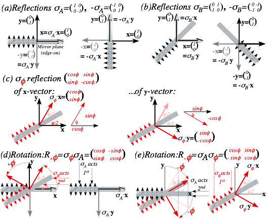
Fig. 5.3 Mirror-reflection geometry (a)±óA, (b) ±óB, (c) óö. Right-and-left-handed rotation (e) óöóA (f) óAóö.
A special case is rotation óA(-óA)=(-óA) óA by ±180° due to setting mirrors at exactly ö/2=90° as in Fig. 5.4b. The result is known as a corner-reflector image. Wherever you stand while viewing a 90° corner you see your image centered and rotated±180° to face you but it is not reflected. A 90° corner image is as others see you, complete with a readable monogram on your jacket and your right hand on the right side.
How fundamental are reflections?
A product of two reflections is a rotation Rö=ó2ó1, but two rotations just give another rotation Rö+è= RöRè and never a reflection. This makes reflections more basic and productive than rotations.
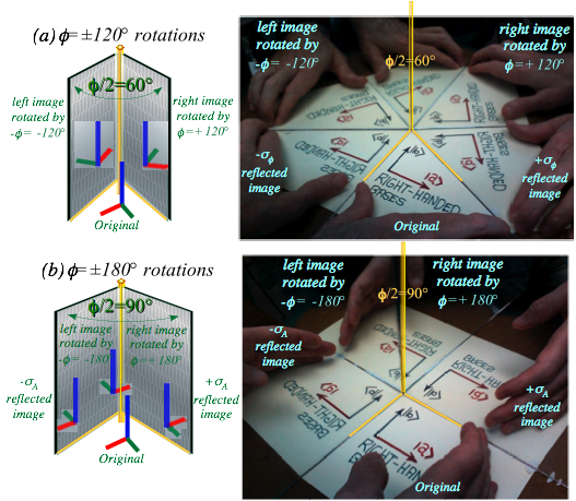
Fig. 5.4 Mirror reflections and their rotations with relative angle: (a) 60° (b) 90° (corner reflector images).
On the other hand, you cannot do a reflection of a real solid object without entering an Alice-in-Wonderland looking-glass-world. Moving every atom in a classical object to a reflected position (without destroying it) is unthinkable! Yet, we easily rotate semi-solid objects (like your eyeballs while reading this).
Waves, on the other hand, are very un-solid and do reflection effortlessly. Rotation takes twice the effort as seen in the looking glass images of Fig. 5.4. This is one reason reflection operations are so basic to the study of wave mechanics, quantum theory, and relativistic symmetry as we will see in later Units. They are elementary symmetry generators in a 1D world. A 1D translation by distance a is two reflections by 1D mirrors separated by distance a/2.
Symmetry
operation R or ó is
defined by what it does to unit vectors ![]() and
and ![]() as óö (5.16) is done in Fig. 5.3c. That matrix
does that same operation to any and all vectors
as óö (5.16) is done in Fig. 5.3c. That matrix
does that same operation to any and all vectors![]() in the
space.
in the
space.
![]() (5.18)
(5.18)
A way to distinguish rotation and reflection operators is by the determinant det|M| of their matrices.
![]()
![]()
A determinant of matrix M quantifies the space (area in this case) enclosed by vectors in M‘s rows or columns (u and v enclose a parallelogram in this case).
A rotation determinant is +1, but a reflection determinant is –1. Reflected area or angle in Fig. 1.3 is negative.
![]()
![]()
Determinants track the multiplication of matrices. The determinant of a product is a product of determinants.
det|M·N|= (det|M|)(det|N|)= det|N·M|
Thus, two reflections each with det|ó|=-1 form a product of det|ó1 ó2|=(-1)(-1)=+1, that of a rotation. This also shows a product of rotations cannot make a negative-det-matrix and so cannot be a reflection.
Exercise 1.5.1 Gameover 49:1
Complete Fig. 5.1 (for m1:m2=49:1) up to the gameover point where sequence would end without 2nd floor bounce. Compare geometric results to analytic matrix analysis.
If the floor is open after the initial bounce of m1, what mass-ratio near that of Fig. 5.1( m1:m2=49:1) would cause m1 and m2 to drop away with the same final velocity.
Exercise 1.5.2 Bigger bangs 100:1
(a) Construct a plot for m1:m2=100:1 to the “gameover” point after which the bigger ball would need a floor bounce to continue hitting the small one. Such a large mass-ratio favors a rescaled (Estrangian) √m1v1 vs. √m2v2 circle–plot. You may use that instead of a plot like Fig. 5.1.
(b) Compare the accuracy of your geometric results with an analytic calculation like (5.2) or (5.13).
Solutions to 1.5.1
Chapter 6 Introducing Force, Potential Energy, and Action
Analysis of force is one of the trickier parts of Newtonian mechanics and one that Aristotle seems to have not done so well. We, like Aristotle, feel we know force after being pushed and pulled around by it most of our conscious lives. Aristotle related force directly to mass and its motion. If he ever wrote equations then, perhaps, Aristotle’s equation would be F=MV.
NOT! MV is momentum, not force. Galileo and Newton may be the first to realize that force should be equated to a change in momentum. A famous equation F=Ma equates force to mass or inertia M times acceleration a, the rate of change of velocity. (It is called Newton’s 2nd law or NEWTON-TWO. Recall (3.16d).)
![]() (6.0)
(6.0)
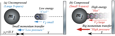
Fig. 6.1 Big mass m1 feels “force field” or “pressure” of small ball rapidly bouncing to and fro.
MBM force fields and potentials
Motion of m1 in Fig. 5.1b suggests a kinetic model and a potential force field. Boltzman uses this to derive gas force laws for volume, temperature, and pressure. As a big m1-ball squeezes space (volume) for a tiny m2-ball in Fig. 6.1, the speed v2 and energy 1/2 m2v22 of m2 increases. So does the momentum transfer rate or bang-force on m1. Energy is related to temperature and bang-force is related to pressure. A furiously bouncing m2 is like a single-atom gas getting hot when its Y-space is compressed as in Fig. 6.1b.
Fig. 6.1 Big mass-m1 ball feeling “force-field” or “pressure” of small ball rapidly bouncing to-and-fro.
A “double-whammy” hits the m1-ball as it closes in with velocity v1 toward m2 and wall (Y=0):
(1) Bang rate B with m2 increases with shrinking distance 2Y traveled by m2 between m1 and wall.
(2) Increased velocity v2 (due to v1) increases momentum m2v2 and ÄP transferred to m1 by each bang.
(3) Increased velocity v2 (due to v1) increases bang rate even more. It’s really a triple whammy!
If m1 is huge (say 1kg) compared to atom or molecule m2 (say (2/3)·10-27kg for an H-atom), the speed v1 of the macro-mass m1 may be negligible compared to typical atomic speeds v2 of 103 m/s. Then we ignore effects (2) and (3) due to tiny v1 in a so-called isothermal model. An adiabatic model includes them.
Atom m2 in Fig. 6.1 travels distance 2Y back & forth between m1 and ceiling at Y for each bang m1. If v1 is slow, the time Ät between bangs is 2Y divided by velocity v2 of m2. Bang rate B is the inverse: B=1/ Ät.
Ät = 2Y /v2 (bangs per sec) (6.1a) B =1/Ät = v2 /2Y (seconds per bang) (6.1b)
Each head-on bang of big m1 on small m2 changes velocity of m2 from −v2 to +v2FIN as shown in Fig. 6.2.
(for: m1>>m2): v2FIN = v2+2v1 (Å v2 for: v2>>v1) (6.2)
Added speed for m2 is 2v1, twice that of incoming m1. (V-V-plot Fig. 6.2 assumes large-m1.) The change ÄP of momentum m2v2 is the difference between FIN value +m2v2FIN and IN value −m2v2.
ÄP = (+m2v2FIN)–(−m2v2)=2m2v2+2m2v1 (Å 2m2v2 for: v2>>v1) (6.3)
So, if “atomic” velocity v2 is large compared to v1 it gives a bang-force F=B· ÄP = ÄP/Ät on m1.
BP= ÄP/Ät =F = 2m2v2(v2 /2Y) = m2v22/Y (6.4)
So a force field F=2·KE/Y on m1 due to m2 is proportional to KE=1/2m2v22 or temperature T of m2. Boltzman’s constant k of proportionality (KE=kT) gives an isothermal force law FY=2kT. It is a 1-D version of Boyle’s ideal gas law: PV=2kT. Here a ceiling tries to keep energy or “temperature” of m2 constant in spite of m1.
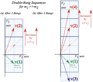
Fig. 6.2 Large mass-ratio (m1/m2>>1) bounce sequence. (Compare to Fig. 4.2a.)
An elastic ceiling can’t give or take energy so each m1 bang adds velocity 2v1 to v2 at rate B=v2 /2Y (6.1). As m1 closes at speed v1 it reduces distance 2Y that m2 travels. So bang rate B grows due to more v2 and less Y.
![]() ,
y =v1t=H-Y,
,
y =v1t=H-Y, ![]() (6.5a)
(6.5a)
We cancel time and v1 to show this force is inverse-Y- cubed, a lot “harder” than inverse-Y in (6.4).
![]() ,
,
![]() ,
,
![]() ,
,
![]() (6.5b)
(6.5b)
This is called an adiabatic or “fast” force law. Collisions are so fast that an isothermal-seeking “Robin Hood” in the ceiling hasn’t time to steal m2’s energy when it’s judged too energy-rich or give energy back when m2 becomes energy-poor. So m2 can get hotter and hit m1 harder and more often as gap Y shrinks.
Conservative forces and potential energy functions
Either force law (5.9) and (6.5) actually conserves the energy of the big-m1 ball in the long run. By that we mean that m1 will come out with practically the same energy that it had when it went in.
The adiabatic case is easier to see. Each bang conserves energy as demanded by the kinetic energy (KE) conservation relation (3.5a). Little-ball velocity v2=const./Y from (6.5b) is used here.
![]() =const. (6.6)
=const. (6.6)
The first term is m1’s kinetic energy KE1. The second term, which is really m2’s kinetic energy, is called m1’s potential energy PE1 or just plain PE, and it is labeled U(Y) since it varies according to height Y of m1 only.
![]() (6.7)
(6.7)
The PE is energy that m1 lends to m2 each time m1 moves a distance ÄY closer so m1 does a little bit of work ÄW on m2. Work is defined as force times distance. (ÄW=F·ÄY) Power, the rate of work done, is defined as force times velocity. Here distance is a small ÄY and the force F in (6.5b) is m2 const.2/Y3. But “work” force might be plus-or-minus (±)m2 const.2/Y3. Which sign? (+) or (−)? Conflicting sign conventions make force-physics confusing. The sign depends on how force and direction are defined. (It’s all relative!)
Is it +or-? Physicist vs. mathematician and the 3rd law
A physicist’s force Fphys is what is felt by a free object (Here that’s m1.) whose motion is driven by force field F=Fphys. A mathematician’s force Fmath is what is needed to hold back the object in the force field. (How apropos! A physicist lets it go but a constipated mathematician holds it back!) They differ by (±) sign only, that is, Fmath =-Fphys, and Fmath is the equal-but-opposite force by an object (m1 here) on its field or force agent(s) (m2 here). (This is essentially Newton’s 3rd law. (NEWTON-THREE) )
Force is momentum flow. Momentum is stuff that’s conserved, so the flow rate Fphys of this stuff into an object m1 must be balanced by an equal-but-opposite negative flow, Fmath =-Fphys, out of the forcing agent(s) (m2 here), and, vice versa, whatever flows out of m1 flows into m2. Momentum p=mv and force F are both vector quantities and a ±sign gives direction to-or-fro, another confusing (±) sign to bother us. But, whatever the flow rate Fphys seen by m1, then m2 sees the opposite rate Fmath =-Fphys.
Let’s define positive Y and F direction to be away from the wall in Fig. 6.1. So incoming m1 has negative velocity v1=-ÄY/Ä t , but after m1 reverses V=ÄY/Ä t is positive. Positive V=-v1 (increasing Y) and positive Fphys means both momentum and energy of m1 are being increased by force Fphys. Each bit of energy or work ÄW=FphysÄY gained by m1 is energy lost by the force-field’s potential “bank” that is m2. (ÄU=- ÄW)
![]() (6.8)
(6.8)
In other words, power Ð =Fphys.V into m1 is power (- ÄU/Ä t ) out of the field. (V=ÄY/Ä t is velocity of m1.)
![]() (6.9)
(6.9)
But is this consistent? Does force Fphys in (6.8) really equal minus the slope of potential (6.7)?
![]() (6.10)
(6.10)
It checks!! Note that F=- ÄU/Ä Y needs that 1/2 on kinetic energy 1/2 m2v22. (Recall discussion of (3.5).)
Isothermal “Robin Hood”and “Fed rules”
The isothermal case is a weird one. The little “force-field agent” m2 maintains it kinetic energy at around the same initial value 1/2 m2v22 no matter how much the big mass m1 loses or gains kinetic energy.
It’s as
though a “Robin-Hood” in the ceiling acts like a big Federal Reserve Bank. (“The Fed.”) Whatever energy m2 earns from m1 is taken and stored away if its over
initial deposit ![]() (m2v22)=T, but if m2 deposits falls below that value, the Fed
makes up the difference. This energy or deposit limit is determined by a
prevailing allowed “temperature” of the ceiling or the current money supply.
(I’m not making this up. It’s what happens in nature and very roughly what
happens in our economy. It becomes a problem if the Fed stops being a Robin
Hood and becomes a robbing hood!)
(m2v22)=T, but if m2 deposits falls below that value, the Fed
makes up the difference. This energy or deposit limit is determined by a
prevailing allowed “temperature” of the ceiling or the current money supply.
(I’m not making this up. It’s what happens in nature and very roughly what
happens in our economy. It becomes a problem if the Fed stops being a Robin
Hood and becomes a robbing hood!)
Under ideal conditions, force agent m2 makes a much “softer” 1/Y force field F=m2v22/Y given by (5.9). Definition (6.9) of force F as negative-U-slope -ÄU/Ä Y then gives a logeY=lnY potential.
![]() (6.11)
(6.11)
It may seem weird that we can define a useful potential while energy-funds are being siphoned in and out. Nevertheless, the ceiling “Robin Hood” is true to his word. (Analogy with “The Fed” ends here!) He puts back all the energy that m1 gave up to m2 (the potential U) on the way in, so that, except for small-change or “tips” left with m2 after the final parting collision, m1 recovers the energy it originally had. Such a force field, if determined by such a reliable potential, is also a conservative one. We discuss later the details of what is needed for general multi-dimensional fields to be labeled “conservative.”
Oscillator force field and potential
Consider a mass m1 between two walls and two little speeding m2 masses as in Fig. 5.5. m1 feels a force like that of an oscillator. As m1 moves distance x off center the left wall space expands to Y+x and the right wall space shrinks to Y-x. Two opposing forces (6.11) then are unbalanced. (Only x2, x4,… terms cancel.)
![]()
Here we let Y=1 be a unit interval and assume an isothermal kinetic
constant ![]() for
each side. For small x (x<<1) the force Ftotal has a linear or Hooke’s law form, and the potential Utotal is quadratic.
for
each side. For small x (x<<1) the force Ftotal has a linear or Hooke’s law form, and the potential Utotal is quadratic.
![]()
![]() (6.12)
(6.12)
Harmonic oscillator
(HO) linear forces and quadratic potentials are, perhaps, the most useful
ones in AMO physics because they approximate any stable system. Normally, they
are analogized by a mass on a spring, rubber band, or pendulum, only rarely (if
ever) in a context like Fig. 6.3. HO motion is sinusoidal ![]() with angular frequency
with angular frequency ![]() and period
and period ![]() independent of
the oscillator amplitude A or phase
independent of
the oscillator amplitude A or phase ![]() . The
calculation of period for Fig. 6.3c is left as an exercise.
. The
calculation of period for Fig. 6.3c is left as an exercise.
The 2nd most useful field is probably the Coulomb potential U=-k/r and force F=k/r2. (See Ch. 7 for electrostatics and Earth gravity, which also have 2D HO potentials at their cores.) After that, the 2D Coulomb U=k·ln(r) and F=k/r is an important field shown in Unit 10. (The latter is like (6.11). A pair of them underlies Fig. 6.3 for the isothermal case.)
You should be warned that an oscillator like Fig. 6.3 is not as simple as it might appear, and as we will see, neither are springs, rubber bands, or pendulums. Also, balls bouncing against moving objects are particularly dicey devices. A simple model with one ball and one oscillating wall is called a Fermi oscillator, and is quite chaotic. The thing in Fig. 6.3 can be even more devilish if m2 is not very small. Caveat emptor!
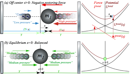
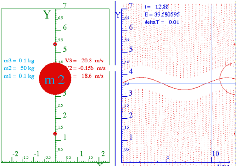
Fig. 6.3 Oscillator force and potential (a) Off center with (-)force (b) On center at equilibrium. (c) Quasi-harmonic oscillation of M=50 in adiabatic force of two m=0.1 masses of speed v0=20 and range Y0=3.
The simplest force field F=const.
We have mentioned power-law forces Fadiab=k/y3=ky-3
(6.5), FCoul=k/y2=ky-2, FisoT=k/y=ky-1 (6.4), and lastly Fosc=-ky (6.12), but have forgotten the simplest,
namely zero power law Fconst=k =ky0. This last one is like a constant
near-Earth-surface gravity force ![]() =
=![]() =mg =-m|g| on a mass m.
( (-) sign for
downward.) Acceleration of
gravity near Earth’s surface is nearly -10 meters per second per second and very nearly –9.8. (g=-9.7997m/s2) Terrestrial objects experience this
whether they are bundled together or not.
=mg =-m|g| on a mass m.
( (-) sign for
downward.) Acceleration of
gravity near Earth’s surface is nearly -10 meters per second per second and very nearly –9.8. (g=-9.7997m/s2) Terrestrial objects experience this
whether they are bundled together or not.
All power-law forces F=kyp have power-law potentials U=-∫F·dy=-kyp/(p+1), except for p=-1 where FisoT=k/y has a logarithmic UisoT=-k
ln(y). (6.11) Earth-surface
potential![]() is linear in height y=h.
This we use to compute height of a superball toss by equating its floor level KE=1/2mV2 to maximum PE=mgh.
is linear in height y=h.
This we use to compute height of a superball toss by equating its floor level KE=1/2mV2 to maximum PE=mgh.
![]() (6.13a)
(6.13a) ![]() (6.13b)
(6.13b)
Ejection height goes as the square of ejection velocity. A 3-fold velocity gain means 32=9-fold height gain.
Introducing Action. It’s conserved (sort of)
It is remarkable that a bouncing mass has a physical
property called action![]() that is more or less constant even if
its position x momentum P and kinetic energy KE
are driven crazy. Action is defined by the area of a one-cycle loop swept out
in a momentum vs position phase-plot
(P
vs x). That is analogous
to an energy or power-plot of force vs position (F vs x)
whose loop area
that is more or less constant even if
its position x momentum P and kinetic energy KE
are driven crazy. Action is defined by the area of a one-cycle loop swept out
in a momentum vs position phase-plot
(P
vs x). That is analogous
to an energy or power-plot of force vs position (F vs x)
whose loop area![]() is work per cycle.
is work per cycle.
Conservation of momentum and conservation of energy are each a rigorously obeyed axiom or theorem for an isolated classical system. However, conservation of action is “more or less” or “sort of” and “it depends” for a driven system. The concept of action is both subtle and deep and it lies at the heart of quantum theory and accounts for a lot of how we affect and are affected by the world around us.
Here we use a geometric construction of a bouncing ball trajectory to quantify action conservation or lack thereof. We suppose the little mass m2 is caught as before in Fig. 5.1 and Fig. 6.1 between a rock and a hard place, that is, bouncing between a big mass m1 (moving in at a constant velocity v1= 1 from the left) and a hard elastic wall. The big ball path is indicated in Fig. 6.4 by a line of slope=1= v1 that hits an initially fixed m2 following a vertical line (slope=0=v2) that then gets knocked up to a line of slope=2=v2 (after Bang(1)). Throughout the imagined collision sequence we suppose the big ball is so much more massive that its change in velocity is not noticeable. This is in spite of the fact that it is absorbing more and more momentum from the little ball with each bang. (Surely, something in it is going to break eventually!)
Each time the small ball is banged elastically by the big one it picks up two more units of velocity v1 that it maintains, apart from change in sign, through its subsequent bang with the elastic wall. Each time it returns for more, is banged again, and increases its speed by two units. (Recall Fig. 6.2.)
The horizontal dashed lines in Fig. 6.4 indicate the range Äx available to the small ball at each instant of its bang with the wall. Note that the product of the range Äx and the speed v2 is a constant three units even as spatial range Äx rapidly decreases and the velocity range Äv=2|v2| increases just as rapidly.
Äx v2 =3.0 = Äx Äv/2
This is an example of conservation of action mentioned before. If we define the small ball’s “range of velocity” by Äv=2|v2| then this relation takes the form of a weird kind of uncertainty relation, that is, it looks like Heisenberg’s famous minimum uncertainty relation Äx Äp =h=(constant) for position and momentum. It happens that the two are related even though the constant used by Heisenberg is an unimaginably tiny Planck constant (h~10-34Js) compared to a constant 3.0 appearing above. (Ours has gadzillions of wave quanta!)
The geometry behind this relation is exposed in Fig. 6.4 (b). It is obtained by considering intersections between lines of integral speeds or slopes v2 =±1, ±2, ±3, ±4, ±5, ±6, ±7,… that are relevant to the bang sequence. They are also relevant to quantum theory where the speeds of a particle in a box are indeed quantized to integers times a tiny number. (This is where that tiny h comes in.) That is simply a reflection (pun intended) of the fact that mutually reflecting waves require that an integral (or half-integral) number of the wavelengths fit perfectly between mirroring containment walls or cavities.
Now we might ask if the action area Äx Äv in Fig. 6.4c-e stays the same if the big-ball speed v1 varies. Action variance was argued hotly by Einstein and the “quantum gang” at the1920 Solvay Conference. They imagined a hotel chandelier being dragged up or down by a clerk holding its support cable upstairs. They concluded that if the clerk could not detect the swinging pendulum phase or frequency, then he would seldom be able to change its action. However, if he could synchronize his oscillations then he could drive the chandelier exponentially to destruction. We shall review this important and explosive process known as parametric resonance in later units. It is fundamental to mechanics and particularly quantum wave mechanics. Action and its wiggly antics deserve our attention.
Monster mass M1 and Galilean symmetry (It’s deja vu all over, again.)
“Monster mass” M1 bongs hapless m2-atoms in Fig. 6.4 using Galilean symmetry. To show symmetry we imagine two head-on monster M1‘s going at ±V1=±1 in Fig. 6.5. A mirror image of Fig. 6.4 lies in extended m2-path lines. The red paths of even integral velocity v2=0, ±2, ±4,… are copies of Fig. 6.4 paths. Odd integral velocity v2=±1, ±3,… paths mesh with even ones to make a full grid. Any initial v2 between ±V1 has a path on the grid. A blue path is drawn thru a series of bongs with v2=-0.2,+2.2,-4.2,+6.2,...in Fig. 6.5.
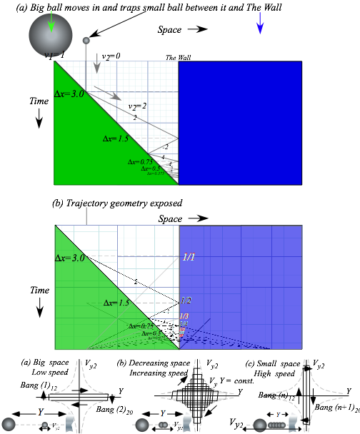
Fig. 6.4 Bang sequence for small ball between big ball and wall. (a) Spacetime paths. (b-c) Geometry of constant product Y·VY of velocity and coordinate ranges.
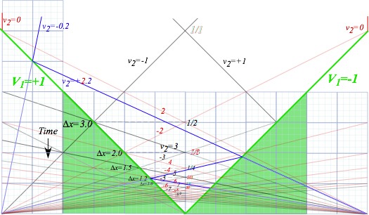
Fig. 6.5 Symmetric pair of head-on V1=±1 monster-m1-masses pong tiny-m2-atoms to higher speeds.
Monster M1/m2-ratios have simple V1-v2-plots shown in Fig. 6.6a. (Recall Fig. 6.2.) Wall M1 simply adds twice its speed (2V1) to incoming speed v2 of atom m2 as M1 bounces m2 out at that speed vFIN2=vIN2+2V1. Monster M1 is the COM so its path bisects in-and-out paths as it balances vIN and vFIN paths of atom m2. (In its COM frame each bong is simply a change of sign for velocity. Recall balance in Fig. 2.6.)
The geometry of adding slope 2V1 to speed v2 is shown if Fig. 6.6a. It is based on the unit square and unit velocity V1=1. Incoming -vIN2 is an altitude of a right triangle with vertical base V1=1, and it is reflected thru the square diagonal to +vIN2 then added to 2V1 to give sum vFIN2=vIN2+2V1 as long side of the triangle with right side vertical base V1=1 in Fig. 6.6a. The hypotenuse is the final path with final slope vFIN2. Each m2-path and slope originates or terminates at base pt-B− or else pt-B+ . These are ends of the double-unit square bisected by unit slope path of M1 terminating at B0. Fig. 6.6.c shows quadrilateral B−B+A+A− bisected by M1 path B0CA0. Similar triangles explain multiple coincidences.
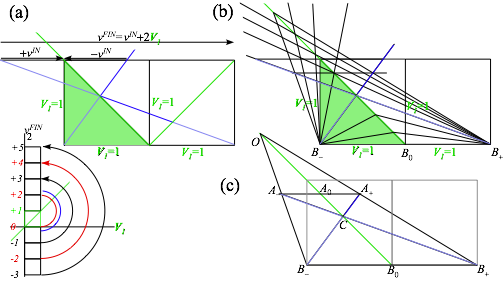
Fig. 6.6 Bisection geometry of Fig. 6.5.
Fig. 6.7 contains time plots for paths in different Galilean reference frames. An excerpt plot in Fig. 6.7a shows how Fig. 6.4 (copied in Fig. 6.7b) appears to a frame traveling at V=1 with each velocity in Fig. 6.7b reduced by V=1 in Fig. 6.7a. Also shown in Fig. 6.7a is the extension of lines connecting the two plots and this highlights this remarkable symmetry. All collision times in Fig. 6.7a match perfectly with ones in Fig. 6.7b though all velocities are shifted. Galileo’s symmetry wouldn’t have it any other way.
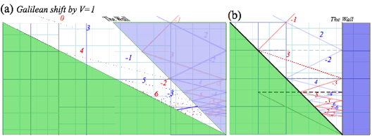
Fig. 6.7 (a) Galilean frame shift by frame velocity V=1 of collision sequence in Fig. 6.4 (shown in (b)).
Exercise 1.6.1 Suppose Fig. 6.3 shows a mass m1=1kg ball trapped between two smaller mass m2=1gm balls of high speed (v2(0)=1000m/s for x=0) that provide m1 with an effective force law F(x) based on isothermal approximation (6.11) while assuming m1 moves only moderately far or fast from equilibrium at x=0.
(a) A further approximation is the one-Dimensional Harmonic Oscillator (1D-HO) force and PE in (6.12). If each mass m2 start in an interval Y0=1m, derive approximate 1D-HO frequency and period for mass m1.
(b) What if the adiabatic approximation is used instead? Does the frequency decrease, increase, or just become anharmonic? Compare isothermal and adiabatic quantitative results for m1=1kg ball being hit by two m2=1gm balls each having speed of v2(0)=1000m/s as each starts bouncing in a space of Y0=1m on either side of the equilibrium point x=0 for the 1kg ball.
(c) How does the frequency decrease or increase in isothermal case versus the adiabatic case if we shorten the run interval Y0=1m to one-quarter meter?…What if we reduce the mass ratio m1/ m2 by one-quarter?
(d) Derive the adiabatic frequency for the case M=50kg in adiabatic force of two m=0.1kg masses of initial speed v0=20m/s and range Y0=3m. Compare with Fig. 1.6.3c.
Exercise 1.6.2 The moving ballwall-trapped-ball constructions in Fig. 6.4 involves a plot of a ballwall coming in with unit slope (velocity). Consider a construction where it has a velocity of 1/2 and intercepts a trapped ball of velocity –1 at space-time point (x=-2, t=4) that is 2 units from the fixed wall. Construct five or more back-and-forth collisions and comment on what, if any, differences exist with Fig. 6.4. If you can, also construct one or two prior collisions (before t=4).
Evaluate approximate or average action values as described in class or after Fig. 6.4 in Unit 1.
Chapter 7 Interaction Forces and Potentials in Collisions
Derivation of force field potentials in Ch. 6 used elementary bangs by tiny m2’s on a big M1. (Ch.5) We predicted elementary bangs between a ball and floor, ceiling, or another ball without knowing potentials. However, three (or more) objects having a ménage a trois are not so easy to predict, and outcomes of 3-body interactions depend sensitively on whatever interaction potential or force law couples the participants.
Geometry of superball force law
When
a superball or any elastic sphere hits the floor or ceiling it dents itself
and, maybe it dents the surface it’s hitting a little bit, too. But, if the
floor, wall, or ceiling is much harder than the ball, we might assume only the
ball develops a “flat-tire” as shown in the Figure 7.1a below.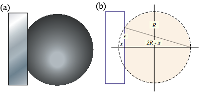
Fig. 7.1 Superball collides with solid wall. (a) “flat” (b) Saggital (“Bow”) mean geometry
The radius r of the ball’s “flat” is indicated by an altitude in Fig. 7.1b and is the geometric mean of the depression distance x and the remainder 2R-x of the ball diameter. (Recall Thales geometry in Fig. 1.9a.)
![]() (7.1a)
(7.1a)
Solving approximately for depression x gives the Saggital (“bow”) formula. (It’s used for thin arc lenses.)
![]() (7.1b)
(7.1b)
How much force F(x) is needed to depress the ball by distance x?
The answer is, “It depends.” A hollow rubber ball or balloon with pressure P pushes back with force equal to product P·A of pressure and area of contact A=πr2. It is a linear (Hooke) force law of a spring.
Fballoon(x) = P·A = P πr2 Å 2πPRx (7.2)
(Recall (6.12) and Fig. 6.3.) Another example is gravity inside the Earth. (See (9.4) or Fig. 9.6 in Ch. 9.)
However, the pressure and force in a solid ball varies non-linearly with x. Even if force varies only linearly with volume of the x-dent in Fig. 7.1b, it’s still non-linear in x. As seen in (7.4) below, sector volume varies roughly as quadratic x2 function. Superballs involve even higher power laws. (Superpower!)
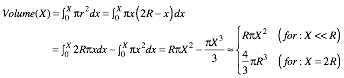 (7.4)
(7.4)
(Here we check that our integral gives the whole ball volume 4πr3/3 for x=2R. That’s the equivalent of crushing the superball into a black hole (or black spot). It’s likely to complain before we get that far!)
Dynamics of superball force: The Project-Ball story
One of the interesting things to come out of Project Ball was the superball’s peculiar force law behavior. The USC mechanical engineering department took an interest in this crazy project when it showed up on NBC News “Ray Duncan Reports.” They offered to measure the superball force curve on a precise tension meter. But, that curve never worked. It didn’t predict the bounces the students were observing. Nothing was making any sense even though we had a big analog computer working it all out.
That was a low point in the project. Even with all this fancy experiment, computers, and theory, I looked like I didn’t know what the heck I was doing. So, what’s new? That’s science most of the time! But, to make things worse we got kicked out of the Project Ballroom, the old basement Lab 69 that we’d squatted in. It was up to be repainted so we had to drag all our stuff out of there and store it down the hall.
Well, after that I had to do something with the students so I arranged for a visit to Whammo Mfg. Co. in San Gabriel, California, where superballs and other goofy stuff was made. The Whammo man said maybe we could talk business about selling our super-elastic toy. So, a day or so later, with $$-signs in our eyes, we piled into our cars and drove down to the plant.
By the time we got there, the inventors were on an all-day “alpha-wave break.” That’s a 60’s fad where you try to increase your creativity by looking at your brain waves. I said, “Maybe, I could use some of that stuff!” But, the company lawyer wanted to show us around. After awhile, he said he thought our invention was cool, but its product liability potential looked too high to make a commercial toy.
We all must have looked pretty sad after hearing that. So he went in a back room and dragged out a big collection of superballs that had been rejected for one reason or another. “Here, take as many as you want!” We thanked him and loaded the balls into some boxes and headed back to USC.
When we got back to Rm 69, the painters were done but the paint wasn’t quite dry. So I said, ”Let’s drop off our new balls so we’re ready for tomorrow.” The students took “drop” to mean literally and dumped them out of the boxes into the empty room. Right away the balls bounced into the wet paint and made lots of little polka-dot spots all over the floor and wall. What fun! What a mess.
Eureka! Polka-dots save Project Ball
But, suddenly, it occurred to me what was wrong with our force analysis and how we might fix it. The engineers had carefully and slowly produced a static or isothermal force curve, but what we really needed was a fast-response or adiabatic force curve. I thought, “Maybe that force law can be told by the polka-dots!”
From a polka-dot radius r made by a superball of mass M and radius R dropped from a height h we could relate gravitational potential energy Mgh to an adiabatic superball potential energy U, and then find a U(x) curve for each value of x=r2/2R in formula (7.1b) by plotting height h against x given by dot radius r. Then the adiabatic force curve F(x) can be found from the slope dU(x)/dx of a U(x) curve.
Just as the adiabatic F=1/Y3 in (6.5) force curve is steeper and curvier than the isothermal F=1/Y in (6.4) so was the polka-dot bounce curve steeper than what we had been using. We stuck our new F(x) on the analog computer’s diode function generator and started getting good predictions. Now we could work out the deadly Model-X3, a 3-ball super tower! (This is described later in Chapter 8.)
First, let’s look carefully at this “polka-dot” potential theory. What we did, like most of physics, was an approximation. Using gravitational potential to estimate superball U(x) is a neat trick only if the superball forces are large and quick compared to the gravitational force or weight mg of the ball.
Fig. 7.2a shows a massive (Bowling-ball sized) superball at its (V=0) drop point h, where potential energy is mgh. Kinetic energy rises from zero as the ball falls and flattens on the floor until it passes a point where the upward floor force cancels the ball’s downward weight mg. That point-xstatic of static equilibrium is at the bottom of the total potential energy curve in Fig. 7.2b. The ball would sit still if put gently at xstatic with no kinetic energy. It’s a point of zero slope since total force F(xstatic) is zero there.
After passing xstatic the ball slows down due to upward force. (That’s positive F(x) for x<xstatic.) Finally it stops at its maximum penetration point xmax where the total energy line intersects the total potential line in Fig. 7.2c. Now the ball’s initial gravity potential mgh0 has been converted completely into potential energy U(xmax) due to compressing rubber a distance xmax. (We’re ignoring tiny frictional heat.)
In the example, the ball’s weight is almost as large as the inertial bang-force driving the ball into the floor. An indication of this is how flat the ball is in Fig. 7.2 b when its weight and compressive force are equal. A standard superball sits stiffly on a table with no noticeable depression, and mg is a tiny part of the total force. It’s so stiff that its bang force is several times its weight and lasts only a few hundredths of a second. Very stiff rebounding potentials are shown in the later Fig. 7.3 and Fig. 7.4 b in which gravity is a negligible force and stiff rebound forces dominate during the collision.
By comparison, the ball in Fig. 7.2 is heavy and its potential is not so stiff. Instead it is so soft it has a big “flat” if sits still with zero KE at xstatic just as it does when passing that point in Fig. 7.2 b. The collision shown in Fig. 7.2 a-c is less like a bang and more like a lingering smooch! Similarly soft collision energy for a linear rebound force and quadratic potential is shown in parts (d) and (e) of Fig. 7.4.
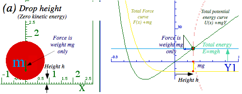
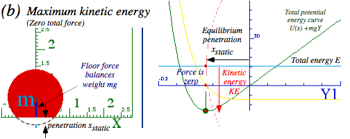
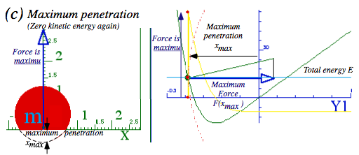
Fig. 7.2 Geometry of ball hitting floor (a) Ball is dropped. (b) Ball at max speed. (c) Ball at low point.
Force geometry: Work and impulse vs. energy and momentum
TV daredevils jump off 30-meter towers and belly-flop into kiddy-pools that are less than 1 meter deep. What a way to earn a buck! And, how do they ever survive such stunts?
Two important physical quantities tell about survival chances. The first is the product F˙x of force-times-distance, or, more precisely, the integral ∫Fdx of force over distance. The second is the product F˙t of force-times-time, or, more precisely, the integral ∫Fdt of force over time. (Recall the fundamental Galileo-Newton relations (3.16) and (6.0).)
The first quantity ∫Fdx is work done or energy -U(x) acquired. U(x) is area under an -F vs. x plot.
![]() (7.5a)
(7.5a)
If energy is stored as potential energy U(x), then force -F(x) is the slope of a U(x) plot at point x.
![]() (7.5b)
(7.5b)
(Recall the discussion of force and potential leading up to (6.10).)
A second quantity ∫Fdt is impulse done or momentum P(t) acquired and area under an F vs.t plot.
![]() (7.5c)
(7.5c)
If momentum is stored in kinetic velocity V(t)= P(t)/M then force F(t) is slope of the P(t) plot at time t.
![]() (7.5d)
(7.5d)
The time equation (7.5c-d) is just Newton’s 2nd law given by (6.0). The space force law (7.5a-b) is just the slope rule first stated (with the physicist’s minus-sign) in (6.9). Both laws deal with conserved stuff. If you, a daredevil, acquire x of this stuff (energy or momentum) sooner or later you are going to have to find something or someone help you get rid of x. Or else!
A daredevil falling 30 meters acquires energy equal to gravity force (body weight Mg) times thirty meters. Fig. 7.3a-b plots a constant F=-Mg and a linear potential U(y)=Mg y from y=30 to y=0. The 1m kiddy-pool must get rid of the 30Mg (Newton meters) of energy in one meter, by applying a force of 30Mg (Newtons) steadily over the entire meter from y=0 to y=-1. (That’s a 30g~300ms-2 deceleration. Human survivability is somewhere around 50g.) An alternative is to get rid of that energy in the concrete below the pool in about 1millimeter, a 30 thousand g deceleration. (That is not survivable!)
Suppose the daredevil falls onto a special trampoline that applies exactly the same constant force as the kiddy-pool, but stores the energy as potential instead of dissipating it all by dousing the audience with a huge splash. (Recall Ka-Bong! versus Ka-Runch! in Ch. 1.) The trampoline could then toss the daredevil back up to the 30 m tower to do the fall over again. (My gosh! What a daredevil has to do to satisfy a sated TV audience these days!) Such a potential is plotted by a steep-slope line U(y)=-30y in Fig. 7.3b.
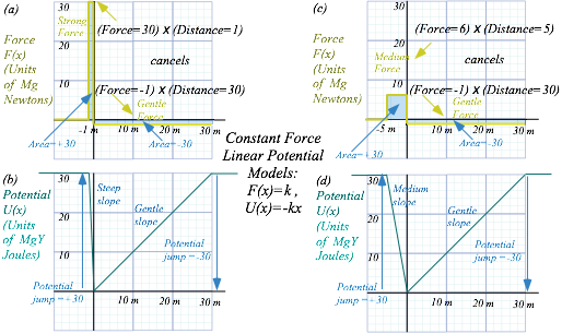
Fig. 7.3 Force and potential plots. (a-b) Strong (30g) deceleration. (c-d) Medium (6g) deceleration.
Suppose the Americans for Humane Daredevilry (AHD) demand that the deceleration distance be increased from 1 meter to 5 meters. (That’s what Olympic divers get for a 10 m fall.) As shown in Fig. 7.3c this reduces the deceleration by a factor of 5 from 30g to only 6g. (A walk in the park!) The sloping U(x) lines are tallying the area-accumulation under the F(x) lines. Starting on the right hand side, U(x) drops by 30 units in 30 meters in Fig. 7.3b to correspond to the –30 units of area under the gravitational F=-1 unit line for the same distance in Fig. 7.3a. The daredevil’s kinetic energy must increase by 30 units to conserve total energy. So trampoline or pool is hit at 24 meters per sec. or 55 mph. (Recall (6.13).)
1/2 M V2=30 Mg or: V=√(60g) = √588=24.2m/sec.
Getting rid of this 30 J potential deficit means climbing a steep 30 J high slope between y=0 and -1 in Fig. 7.3b or a medium slope of the same height between y=0 and –5 in Fig. 7.3d. Both cases have the same +30 J area under a force line, but having 5 meters instead of just one reduces the force to 30/5=6.
Time functions F(t) and MV(t)=P(t) relate to F(x) and U(x) using Newton II: F=MdV/dt in (7.5d).
![]() or:
or: ![]() (7.6a)
(7.6a)
![]() or:
or:
![]() (7.6b)
(7.6b)
The first relation is total energy conservation (KE+PE=const.) first stated in (6.6) and (6.7).
Linear force law, again (But, with constant gravity, too)
Let’s imagine the AHD demands further protection of daredevils from themselves by outlawing constant-force targets that turn on a full force suddenly upon entry. Claiming that “high-jerk” is bad, the AHD requires linear-force targets, instead. Physicists comply happily since a harmonic-oscillator linear-force-quadratic-potential (6.12) is the favorite force law. It also describes inside-Earth oscillation in Chapter 9.
Plots of linear-force-quadratic-potentials are shown in Fig. 7.4. Just like the preceding Fig. 7.3, a constant gravitational force Fgrav=-Mg is present both in and out of the (y<0)-region where the linear F=-ky force and the U(y)=1/2ky2 potential exist as a sum of constant and linear forces for (y<0).
![]()
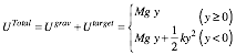
(7.7a) (7.7b)
If a linear potential b·y is added to a quadratic a·y2 potential we get the same parabolic curve U=a·y2, but that curve is shifted to the left by yshift=-b/2a and down by Ushift=-b2/4a as follows.
![]() (7.8a)
(7.8a)
![]() (7.8b)
(7.8b)
The nose or tip of the parabola, which is the equilibrium resting point, follows an upside-down copy of the U-parabola itself! This important geometric fact is shown in Fig. 7.4. The geometry does not reveal itself until we look in Fig. 7.4e at a “soft ball” that is soft enough to clearly show its gravitational shifts. A hard superball is more like Fig. 7.4b that barely shows such a small shift.
Hardball total potential is u(y)=8y2+y with a total force function f(y)=-16y-1 in graph units of Fig. 7.4(a-b). A medium total potential is u(y)=y2+y with a total force function f(y)=-2y-1 is plotted in Fig. 7.4(c-d). The latter clearly shows the equilibrium or lowest “sag” point of zero force. The softball total potential is u(y)=(1/4)y2+y with a total force function f(y)=-(1/2)y-1 in Fig. 7.4e. The hardball potential requires about 6 meters (Y=-6 or y=-0.6) to cancel the energy from the 30 meter fall (from Y=30 or y=3) and maximum force of about F=10. This is much more than the constant F=6 that stopped the same daredevil in 5 meters in Fig. 7.3c because a linear force has only the area under a triangle which has a factor of 1/2. Here 1/2(F=10)(Y=-6) gives the necessary energy of 30 Joules. So the AHD ruling has actually increased the maximum force on the daredevil! (But, only during the final milliseconds is F large.)
Note that the focus of the U(y) parabola is on the y-axis because we plot gravity with slope=1. Can you find a geometrical a way to locate that focus given some allowed stopping distance?
Parabolic geometry of an oscillator potential subject to a uniform (or nearly uniform) force field is an important one in physics. Electronic charges pinned to an atomic potential well behave like oscillators in an electric field of a passing light wave. Generally the light wavelength of 0.5 micron (0.5E-6m) is several thousand times as long as the atomic radius of a few Angstrom (1E-10m). So the effective potential is a rigid parabola like Fig. 7.4e shifting to and fro and up and down at some frequency.
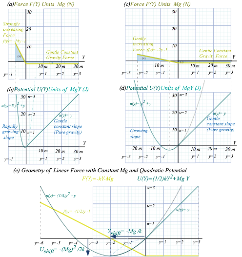
Fig. 7.4 Linear deceleration force after constant falling force. (a-b) Hard (c-d) Medium (e)Soft
As
we mentioned, superball force function is non-linear; approximately Fball(y)~y4
plotted in Fig. 7.2 and Fig. 7.5 below. Compare this to the linear balloon-like
force curve Fballoon(y)~y1
in Fig. 7.4e above. (Recall (7.2).) Fballoon(y)
is a pair of straight lines bent at contact point y=0, while
Fball(y) has a long flat region below y=0. For either case, the force integrals ∫Ftotal(y)dy and
the areas they represent cancel between any two points y=h and y=ymax
that have the same potential energy U(h)=E=U(ymax).
If that energy is the total energy E
then these points y=h
and y=ymax
are classical
turning points. The mass M
stops with zero KE
(no speed) to turn around and fall backward or forward, respectively, into the
potential valley lying between h
and ymax. PE curve Utotal(y) near
bottom (ystatic)
in Fig. 7.2-5 is nearly parabolic as is U(x)
in Fig. 6.3. The difference for Fig. 7.4 is that all
of the Utotal(y)
curves are perfectly
parabolic for y<0.
(See exercise 1.7.1.) 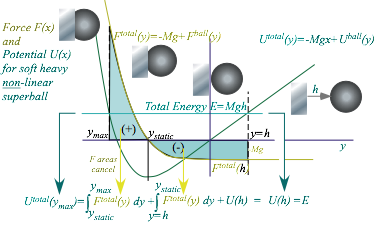
Fig. 7.5 Force and potential for soft nonlinear (F=ky4) superball dropped from height h
Super-elastic bounce involving two balls was introduced way back in Fig. 4.5 and “explained” by the 2-Bang model sketched there. Is that the only explanation? Certainly not! Is it even right? Well, yes and no. Here is a chance to discuss how science works or doesn’t work. It is, after all, a human endeavor. (To err is…)
Let’s imagine a big scientific fight between two research groups something like real ones I’ve seen. We’ll imagine it’s about superball dynamics. On one side is a small but creative group working for the Rumpany Company® that first discovers the effect and explains it with the 2-Bang model. But their small budget limits them to things you can do cheaply with a ruler and compass.
On the other side is the huge Crap Corporation®. With unlimited military contracts, CrapCorp can afford any kind of computer or lab equipment. They hear about RumpCo’s discovery and decide to develop and sell it to the Army as a bomb detonation system.
I hope you’ll excuse a scatological nomenclature and contempt for shortsighted and mindless goals often associated with post-modern cash-flow-science. My allegorical objective is to encourage curiosity-driven-science that is now becoming regarded as quaint. I do believe that humans are capable of creating much more than fertilizer and should be strongly encouraged to do better. If earning gets in the way of learning, then humans do poorly. I have watched big labs in government, industry, and university die of a pernicious groupthink fueled by the acquisitive rather than the inquisitive human drives. People lose their ability to reflect and become happy to merely genuflect. A novel Radiance by Carter Scholz (Picador 2002) is a “Star Wars” romaine a’clef exposing foibles of scientists at Livermore and Los Alamos.
On one side of our allegory is poor but resourceful little RumpCo full of ideas but nowhere to go. Their 2-Bang model of super-elastic bounce is simple, elegant, but appears wrong. The powerful CrapCorp, on the other hand, knows where it’s going and what’s right. It has every resource imaginable. Except wisdom.
CrapCorp’s first move is to discredit RumpCo’s work. They set up a computer that uses lab observed potential functions to fully analyze a 2-ball bounce. Let’s compare two competing vu-graphs side-by-side.
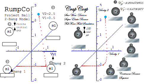
Fig. 7.6 RumpCo theory versus CrapCorp’s simulation. (RumpCo) Finite initial gap (CrapCorp) NO gap
One thing is clear. CrapCorp does fancy-schmancy vu-graphs! They resemble wedding invitations.
And, while CrapCorp’s 10-figure precision is dubious, we note their V1=0.62 and V2=2.29 disagree with RumpCo’s predictions (Recall Fig. 4.4.) of final V1=0.5 and V2=2.5 by a little. Furthermore, RumpCo uses an independent 2-ball bang model. They assume or idealize an initial gap separating mass m1 from m2 so Bang-1 of m1 with the floor is independent of Bang-2 between m1 and m2. So V1 and V2 result from 2-body energy-momentum conservation. RumpCo’s results are not sensitive to force functions.
CrapCorp can compute the difficult 3-body collision between m2 , m1, and m0 (the Earth) all together just like what’s really happening on the floor. CrapCorp ‘s curvy V1 vs. V2 plot in Fig. 7.6 is very sensitive to each force function F(y) between each pair of colliding bodies. When (and if) CrapCorp values check out with experiment, they’ll happily sneer at the primitive pair of straight lines in the RumpCo velocity plot.
Does RumpCo have nearly the right (V1,V2) for wrong reasons? Not entirely. The reason a 2-Bang model works at all is that the force function for these balls is highly non-linear. A quartic function F(y)=y4 has a flat bottom as noted before Fig. 7.5. That allows the floor-m1 collision to nearly finish before the m1-m2 bang really gets going even though the balls are in contact all during the collision.
Realizing this, the RumpCo researchers suggest that CrapCorp try a linear force F(y)=y1 simulation to see if super-elastic bounce disappears. They do, it does, and the rest is history. As seen in Fig. 7.7, m1 and m2 bounce up in unison. It’s a pax de deux. Super-elastic bounce goes away!

Fig. 7.7 Linear force kills super-elastic bounce. (Collaborative effort.)
The two groups decide to stop feuding and join forces. A corporate merger results in a multi-national conglomerate Carumpany Ltd. based in the Caymans. They lived happily ever after. (Well, sort of.)
Another important physics lesson from this section is, “Fasten your seatbelts…tightly!” To avoid great and damaging force you need to avoid non-linear force functions and fasten yourself with linear ones that can start working off your kinetic energy and momentum most immediately after a collision. The non-linear force with its “flat” region applies little or no force at first but then has to make up for its procrastination with deadly high force after it’s too late. Note how nonlinear force in Fig. 7.5 finishes much higher than the linear force in Fig. 7.4. Even worse is having no seatbelt at all. That’s like a very non-linear force of, say, F(x)=kx100. It’s a flat gap with a practically vertical wall waiting to crush you!
One of the most dangerous vehicles in the Wild West of the early US was the buckboard, a wagon with no suspension except for a set of springs right under the rider’s seat. When the buckboard hit a bump it generally lived up to its name. Unfortunate riders ended up like a little m1 superball knocked skyward by a big m2 wagon. A safer and more comfortable ride is had in a car with a body as much heavier than the wheels and suspension as possible. So-called “Monster trucks” have the worst kind of ratio possible for stability.
Friction and all that “dirty” stuff
Slowly we have put back some of the “real-world” features of the superball collisions that our idealized “Bang-Bang” models of Ch.4 ignored in order to make the problems more easily solvable. The effects of gravity during collision have been introduced and applied to interacting zero-gap superballs.
More such effects will be studied in what follows since interacting linear forces are very common in nature and there are ways to make them easily solvable, too. The oscillating neutron star in Ch. 9 provides a taste of what is to come in the study of waves and oscillation in Unit 4 and orbits in Unit 5.
But even the neutron star model neglects what is the bane of the purist physicist, the dreaded frictional forces. These are among the most neglected and poorly treated physical effects in physics. If anything goes wrong with a theory, we just blame it on friction! Often we have little choice in this matter.
Friction is a result of having more particles than we’d like to admit. Consider one m1=72 gram superball. That’s about a mole of Carbon C6 rings and a mole has 6.02E23 (That’s Avogodro’s number.) of these C6 molecules. So we’re dealing with not one mass m1 particle but an enormous heap with an unimaginably huge number 60,200,000,000,0000,000,000,000 of particles that individually are (mostly) friction-free and well behaved, but their mob-behavior is just plain abominable!
You’ve got to get down to at least the individual molecular level before “internal-friction” is pretty much a non-existent phenomena and pure quantum wave mechanics rules. So what we call “frictional loss” is simply the best accounting we can do of 60.2 gazillion chiseling thieves stealing bits of energy that turn up later as “heat.” In conservative economics the effect is known as “supply side” or “trickle-down.” Let’s see if we can account for energy chiseled by just three thieves. (And, then we’ll hire more thieves until we bankrupt the whole operation!)
Important atomic and molecular force geometry
1.1.2 A most important mechanics problems is that of atomic oscillators affected by electric fields since it is basic to all spectroscopy. A useful approximate model is potential Vatom(x)=k x2/2 function of center x of charge Q where k is a spring constant of atomic polarizability. A uniform electric field E is assumed to apply a force F=Q·E to the charge by adding a potential VE(x) to Vatom(x). (Give VE(x)=______ and FE(x)=_____)
Consider the resulting potential Vtotal(x) for an atom for unit constants k=1 and Q=1. Derive and plot the new values for equilibrium position xequil(E), energy Vequil(E), dipole moment pequil(E). Plot Vtotal(x) for field values of E=-2,-1, 0, 1, and 2.
Does charge oscillation frequency ùequil(E) change? If so express in terms of ùequil(0) and E?