Chapter 9 Geometry and physics of common potential fields
Physical and geometric aspects of elementary force and potential fields are introduced in this section. Most important are oscillator and Coulomb fields that will later occupy Unit 4 on resonance and Unit 5 on orbits.
Geometric multiplication and power sequences
The most common power-law potentials are U(x) = Ax2 (Oscillator potential) in Fig. 9.1, U(x) = Ax (Uniform field potential) , and U(x) = Ax-1 (Coulomb potential) Fig. 9.5. Power-law potentials and force laws have simple geometric constructions. Exponential or logarithmic fields (shown in Ch. 10) do not.
Multiplicative power operations are done using a staircase of similar triangles as shown in Fig. 9.2. A geometric progression {1=s0, s=s1, s2, s3,…} and an inverse progression {1=s0, 1/s=s-1, s-2, s-3,…} lie on either side of the unit stair step 1=s0. A slope or scale factor s=2 or s=1/2 is used in Fig. 9.2a or Fig. 9.2b. They resemble perspective drawings of school hallways. (Elementary School is (a) and High School is (b).) Each stair zigzags between slope-1 line-(y=x) and slope-s line-(y=s·x) or between line-(y=-x) and line-(y=x/s). The line-(y=s·x) and line-( y=x/s) are perpendicular or normal to each other. So are line-(y=x) and line-(y=-x).
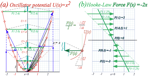
A two-step triangle in Fig. 9.1a gives each point on the oscillator potential, a parabola y=x2. To find where the parabola hits vertical line-(x=2.2), for example, we go up that line to the 45° line-(y=x) and then go across to vertical line-(x=1). A dashed blue line is drawn from origin thru that point to an arrow intersecting line-(x=2.2) at pt-(x=2.2, y=2.22) on parabola-(y=x2). A similar zigzag gives pt-(x=-2, y=4) or any point on the parabola (y=U(x)=x2) below.
Fig. 9.1 Geometric construction of U(x)=x2 potential and Hooke’s force law F(x)=-2x.
The
physicist Force =-Slope
rule (6.9) is drawn using force triangles in Fig. 9.1a. Force is linear in x, that is, F=-2x, and that is minus the slope of x2. A line of slope –2 in Fig. 9.1b plots F(x). Force vector F scaled by 1/2 gives a force vector shown in Fig. 9.1a
equal and opposite to coordinate x. Each force triangle has base F/2, an altitude that is a constant 1/2, and a hypotenuse normal to the parabola
tangent. It is similar to the tangent triangle with base ÄU and altitude Äx (center of
Fig.9.1) that shows force=-slope (![]() ).
).
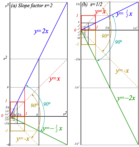
Fig. 9.2 Geometric sequences and “staircases” for slope or
scale factor (a) s=2, and (b) s=1/2 .
Parabolic
geometry
A parabola U(x)=Ax2 has a focal point at y=U=A/4 where vertical rays meet if reflected by parabola tangents as in Fig. 9.3b. A parabolic radius is its half-width ë at the focus. For y=x2 we have ë=1/2. (Note how F(±0.5) vectors point at the focus in Fig. 9.1a.) An old name for ë is latus rectum. A circle through the focus about any parabolic point will be tangent to a line called the directrix located at a distance ë from the focus. Focus and directrix define a parabola that passes midway between them thru the tip-point M of the parabola where its focal radius and equal distance-to-directrix both reach their minimum value ë/2.

Fig. 9.3 Parabola and analytic geometry (a) Rays converging on focus. (b) ë-geometry of tangent reflection.
Directrix is a so named because it “directs” both the rays and wave phase of an optical reflector. Since the focal radius (length of each sloping ray line in Fig. 9.3a) equals the perpendicular directrix distance (length of corresponding dashed vertical line), waves are guaranteed to be plane waves. Also, the equality of angle of incidence and reflection off the parabola bisecting the dashed and solid lines, guarantees vertical parallel rays for all which leave the focus and bounce off the inside of the parabola. It also guarantees that parallel vertical rays bouncing off the outside will go away from the focus. Either side of a parabolic surface converts plane waves to spherical ones or vice-versa.
To
better understand the parabola’s geometric optics we draw examples of the tangent-kite
for four different tangent slope values. The blue kite of slope=2
in Fig. 9.4a and yellow kite of slope=5/2 in Fig. 9.4b have equal focal radius and
perpendicular distance-to-directrix forming the major iscosoles triangle of the
kite. A minor iscosoles triangle (upside down in Fig. 9.4) shares a base with
the major one. Their perpendicular bisector is the tangent line. The bisection
point is slope![]() in
units of ë as
indicated by vertical arrows.
in
units of ë as
indicated by vertical arrows.
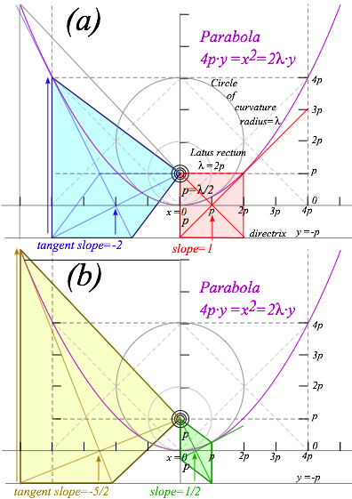
Fig. 9.4 Parabola and geometry of curvature and slope of tangent-kites.
A singular case is the red kite of slope=1 that is square. Lesser slope=1/2 gives a rhomboidal green kite with one side on the vertical parabolic axis instead of on the horizontal directrix. Points of slope=±1 on the (4py=x2=2ëy)-parabola lie on either side of its focus at distance ë=2p from it. ë=2p is also the (minimum) radius of curvature of the parabola at its tip (minimum y at x=0) that lies a distance ë/2=p below the focus.
Coulomb and oscillator force fields
Our atoms and molecules depend on the electrostatic Coulomb field to have stable chemistry and biology. Like charges repel and opposites attract with a force that varies inversely with the square of distance r between them. A simple version of the electric Coulomb force law (axiom) is:
![]() (9.1)
(9.1)
The units and notation are standard but the size of this is mind boggling. It’s nine billion Newtons for
just two charge-units a meter apart. (To be precise it’s 8.99·109
Nm2/C2.) OK, a 1N is only about ![]() lb, but
are you able to hold up a billion sticks of butter? Also, you have thousands of Coulomb charge
units in each fingertip with only a centimeter separation so add another factor
of (100)-squared.
Make that ninety trillion
Newtons for each Coulomb or about a million
trillion Newtons trying their darndest to blow your pinkie to bits!
lb, but
are you able to hold up a billion sticks of butter? Also, you have thousands of Coulomb charge
units in each fingertip with only a centimeter separation so add another factor
of (100)-squared.
Make that ninety trillion
Newtons for each Coulomb or about a million
trillion Newtons trying their darndest to blow your pinkie to bits!
But, still we’re underestimating this monster force. Most of the electronic charge in the world is crammed into atoms and molecules with at most a nanometer (10-9 meter) across and some are an Angstrom (10-10 meter) or a tenth of a nano. So put on another factor of (10-9)-squared or million-billion trying to undo your pinkie, that’s a trillion-trillion-billion. Does your manicurist know about this?
Sometimes these forces get loose as in a TNT blast, but usually, tiny nuclei with an equal positive charge hold down potentially rebellious electrons. Still, what’s holding nuclei together? Nuclear radii are femto-meters (10-15 meter) or Fermi. (Note: both fm and Fm are abbreviations for 10-15m=10-13cm.)
Oops! That’s another factor of (10-15)2 or another million-trillion-trillion to increase our stress level. Nuclear charge is 105 times more pent-up than its atomic electronic counterpart with a grand total of about a trillion-trillion-trillion-trillion Newtons hankering to blow up your fingertip nuclei. Cancel the manicure!
When nuclei do blow up, the result is more than 105 times more devastating than TNT bangs. We don’t use force to estimate the devastation of a nuclear fission bomb or the yield of nuclear power plant fuel. Rather we use electric potential energy, that varies as 1/r not 1/r2. (Slope of a U(r)=1/r-curve is F(r)=1/r2.)
![]() (9.2a)
(9.2a)
Energy or (Force)-times-(distance)-unit is Joule or Newton. meter (N·m). Like superball potential field U(r) in (6.9), force F(r) (9.1) is a (-)derivative of potential U(r) that in turn is (-)integral of force F(r). (Recall (7.5.)
![]() (9.2b)
(9.2b)
![]() (9.2c)
(9.2c)
Potential nuclear energy yield is about a million times greater than for the same number of chemical energy sources since femto-meter nuclei are a million times smaller (RNUC~10-15) than nano-meter molecules (RMOL~10-9). Nuclear forces would then be a trillion times greater than typical atomic and molecular forces.
Fig. 9.5 plots attractive Coulomb force F(r)=-1/r2 and potential U(r)=-1/r of negative charge -q to a positve +Q nucleus. (Negative force points toward the +Q origin (x=0).) It uses zigzag geometry of Fig. 9.4.
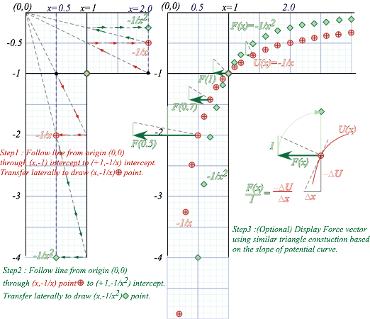
Fig. 9.5 Attractive Coulomb force F(x) and potential U(x) curves. (F(x) vectors drawn at 1/4-scale.)
Could the Coulomb F(r)~1/r2 force field be derived like the superball force F(Y)~1/Y3 in (6.10) by counting momentum bangs? Indeed, if a charge ejected a cloud of little “bang-balls” then the number of bangs scored at distance r would vary inversely with area 4πr2 of a radius r sphere. But, that idea doesn’t explain very well attraction of a charge +Q to a –q or of a mass M to a mass m in Newton’s gravity law.
Fgrav(r) = -GMm / r2 , where: G=0.000000000067 N m/kg2 (9.3)
Gravity is universally attractive (no “negative” matter
readily available) but much weaker than the electric one since G constant 6.672E-11 (![]() in mks units) is smaller (by 1020
times!) than the
in mks units) is smaller (by 1020
times!) than the ![]() in
(9.2).
in
(9.2).
As of this writing it is still a mystery why these are so different. We really do not yet understand either of these forces at a fundamental level. They are still very much in the axiom box.
Tunneling to Australia: Earth gravity inside and out
Imagine x=1 in Fig. 9.5 is the Earth radius R⊕=6.4E6m. The F(r) plot shows gravity falling off for r>R⊕or x>1. But it’s wrong for subterranean radii (r<R⊕) unless Earth is compressed. F(r)=-1/r2 doesn’t apply everywhere unless Earth is squashed to a 10 millimeter radius “black hole.” (More on this later.)
If you were to be at sub-R⊕ levels all Earth mass at radii above your radius r can be completely ignored in figuring your weight! As you might expect, you’re weightless at the center (r=0) since the pull of all Earth’s mass exactly cancels there. But, so also does your attraction to a spherical mass shell cancel anywhere inside it. One could float weightlessly anywhere therein regardless of the shell’s size or weight.
Such a cancellation is a geometric peculiarity of an inverse square law. (It also underlies a Gauss law explanation of why you’re safe inside a car struck by lightning.) Any direction you look inside a uniform mass shell has a mass element m whose force is cancelled by another element M behind. (See Fig. 9.6.)
The shell tangent to the m-point you’re facing intersects the tangent to the M-point behind you to make an isosceles triangle whose sides make an angle È with your line of sight along the base. This means a narrow cone of sight will include shell mass m=Ad2 at a distance d in front of you and shell mass M=AD2 at a distance D directly behind you, where the angular factor A~1/sinÈ is the same for both. That assures perfect cancellation of gravity m/d2 in front with -M/D2 behind you. This applies for all directions in Fig. 9.6.
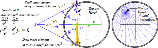
Fig. 9.6 Equal-opposite attraction. Geometry for you floating weightless inside a spherical shell.
A mass m at radius r inside Earth feels gravity attraction GmM</r2 where M< is Earth mass inside the radius r indicated by the dashed circle in Fig. 9.6. If Earth is uniform density ñ, then that inside-mass is M<=4 ñπr3/3. Force law r-2 cancels all but one r of the r3 in mass M<. We then get a linear force law.
Finside(r)=GmM</r2=m(G4πñ /3) r=mg(r/R⊕)=mgx (9.4a)
(Earth surface gravity: g= G R⊕4πñ /3=9.8ms-2) (9.4b)
The linear force law (9.4) is like that of a harmonic
oscillator in Fig. 9.1b and so the inside-Earth potential must be a parabola
like Fig. 9.1a. Force F(1)=-1
is continuous as we cross x=1
and so must be the slope of potential U(x)
as U changes from –1/x2 to
parabola. Terrestrial beings such as ourselves live in a nearly-constant-field
(![]() )-region
near x=1. In Fig. 9.7
we find the potential parabola geometrically by its focal point and directrix
using the tangent at x=1.
Recall a tangent at x=ë=2p in Fig. 9.4a has slope=1 or 45°.
So does the parabola at x=1
in Fig. 9.7 below have a slope of (+1) and a force of (-1) (That’s –mg
in mks
units.)
)-region
near x=1. In Fig. 9.7
we find the potential parabola geometrically by its focal point and directrix
using the tangent at x=1.
Recall a tangent at x=ë=2p in Fig. 9.4a has slope=1 or 45°.
So does the parabola at x=1
in Fig. 9.7 below have a slope of (+1) and a force of (-1) (That’s –mg
in mks
units.)
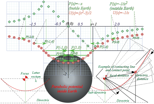
Fig. 9.7 Construction of Earth gravitational fields inside and outside.( units of x: R⊕,; F: mg; U: mgR⊕)
A parabola tangent bisects the angle between the line to the focus and the directrix drop-line as in Fig. 9.4. Twice 45° gives 90°. The focus is ë=1.0 units straight across and the directrix is ë=1.0 units below as shown in Fig. 9.7 (lower-left). Using this we may construct the parabola by rotating a square corner of a piece of graph paper around the focus so the corner touches a line halfway to the directrix. (We can call this half-way line the sub-directrix. It is the line of tangent intersections indicated by arrows in Fig. 9.4.)
The parabola so constructed is y=x2/2 –3/2. That is the interior potential UIN(x) (-1<x<1). It meets the curve y=-1/x that is the exterior potential UEX(x) (1<x<∞) at x=1 where they are equal (UIN(1)=-1=UEX(1)) as is slope, which is the force (FIN(1)=-1=FEX(1)). (However, the slope of the force curve takes a big jump!)
Adding
a constant to a potential won’t alter slope or force. We added ![]() to
to ![]() to make it equal
to make it equal![]() at x=1.
at x=1.
To catch a falling neutron starlet
The “glue” that holds in the rebellious nuclear proton charge is called nuclear matter, a mix of neutrons, mesons, and their ingredients. Let’s imagine a fingertip (1cc) of neutrons as densely packed as they are in a nucleus or neutron star and estimate how such a neutron starlet might travel through Earth. First, we find the density of nuclear matter. Let’s say a nucleus of atomic weight 50 has a radius of 3 fm, so it has 50 nucleons each with a mass 2·10-27kg. (It’s actually more like 1.67·10-27, but roughly 2·10-27.)
That is 100·10-27=10-25 kg packed into a volume of 4π/3r3= 4π/3 (3·10-15)3 m3 or about 10-43 m3. That gives a whopping density of 10-25+43 = 1018kg per m3 or a trillion kilograms in the size of a fingertip.
That’s a pretty heavy fingertip! Its weight mg is ten trillion Newtons. (Well, actually 9.8 trillion Newtons. No need to exaggerate here!) In spite of this, its gravitational attraction to nearby rocks on the Earth is comparatively moderate. A (10cm)3 1kg rock would cling to the starlet with a force of about
Frock=Gm(1kg)/r2= 100Gm = 100(6.7E-11)1E12 = 6,700 N, (m=Mstarlet=1012kg)
or less than a ton and small change for a starlet weighing billions of tons and cutting into the Earth like a bullet going through cotton candy. Let’s see what speed it might gain falling from the surface.
Starlet energy is assumed constant since friction would be tiny compared to its enormous weight.
E = KE + PE = 1/2 m v2 + U(x) =1/2 m v2 + 1/2 mg (x2 –3)=const. (9.5)
Let it be released at Earth surface (x=1) with zero velocity. This sets the energy constant.
E =1/2 m02 + 1/2 mg (12 –3)=const.=- mg (9.6)
At Earth center (x=0) we solve for the velocity there. (The starlet mass m cancels out.)
E =1/2 mv2 + 1/2 mg (02 –3)=const.=- mg or: v2 = g , (9.7a)
v = √g (In mks units: v2 = gR⊕ , or : v0 = √(g R⊕)=8 km/s) (9.7b)
v0 = 8 km/s is also Earth’s minimum orbital insertion speed. A mass dropped down the tunnel flies with the same x-coordinate as one shot with the speed v0 into circular orbit. One flies above the other and they meet each other on the other side 42 minutes later as shown in Fig. 9.8. We now show this synchrony of orbital timing holds for all pairs of starlets sent from anywhere inside the Earth!
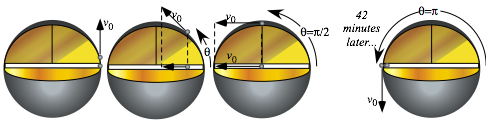
Fig. 9.8 Neutron starlet penetrates Earth as satellite orbits to meet 1/2-way around in 42 minutes.
This synchrony involves a physicist’s most favored type of potential energy U=1/2kx2. When PE=U is a square like kinetic energy KE=1/2mv2 we have a wonderful symmetry between position x and velocity v.
E=KE +PE= const. = 1/2mv2 + 1/2kx2
We make any constant-sum-of-squares into a Pythagorian relation 1=sin2è+cos2 è just as we did to analyze the sum (5.10) of super-ball KE. Here (9.5) is a sum E=KE+PE and the constant k is starlet weight mg.
1=(m v2/2E) + (k x2/2E) =sin2è+cos2 è (9.8a)
Position x and velocity v are then expressed in terms sine and cosine of a phase angle è .
x= √(2E/k) sinè (9.8b) v= √(2E/m) cos è . (9.8c)
Velocity v
is proportional to cosè and è has a constant angular velocity ù=![]() so that è=ù·t+á. (á=è0=const.)
so that è=ù·t+á. (á=è0=const.)
![]() (9.9a) where:
(9.9a) where: ![]() (9.9b)
(9.9b)
Angle è is a polar angle in (x,v/ù)-phasor-space of Fig. 9.10a. (x,v/ù)-orbits are circular-clockwise (ù=−|ù|) if positive phasor v-axis is up and positive-x axis is to the right. Earth xy-orbits may be elliptical with a polar angle ö that can orbit either way in Fig. 9.10. Each spatial dimension x and y has a constant sub-total energy.
KETotal=ey+ey where: ex=const.= 1/2mvx2 + 1/2kx2 and: ey=const.= 1/2mvy2 + 1/2ky2 (9.10)
Equal constants (ex=ey) give the circular orbit in Fig. 9.8. Frequency ù (9.9) is independent of energy value ex or ey and so orbit and x-tunnel motion each have frequency ù=√g, but tunnel motion, with same ex but zero ey, has half the energy. All motions of the starlet inside the Earth have the same 84-minute period. That is a fundamental harmonic period of a uniform Earth and approximates behavior of the real Earth.
To depict the force vector F on
the starlet simply draw an arrow from it to origin as in Fig. 9.9a since F is proportional to coordinate vector -r. (In Fig. 9.7, F is equal to –r.) It’s projection on x or y-axes are the forces components driving
the 84-minute oscillations along x or y-axes. Perhaps, there is a starlet deep
below us swishing out 84-minute elliptical orbits as in Fig. 9.9b. 
Fig. 9.9 Force and orbits inside Earth. (a) F is minus the coordinate vector (b) Typical orbits.
Starlet escapes! (In 3 equal steps)
Imagine starlet-m has decayed to where it sits at the bottom of the U(x)=1/2mg(x2–3) curve in Fig. 9.7. How much energy does it take for it to escape from Earth center and go back whence it came? The plot of U(x) in Fig. 9.7 and discussions above suggest three equal steps of 1/2 that bring energy -3/2 at x=0 up zero at x=∞
Step-1 is to drag or shoot the starlet-m to the Earth’s surface. That takes energy ÄE1=1/2. (That’s 1/2mgR⊕ in mks units.) Shooting radially at velocity v0 = √(gR⊕) given by (9.7b) would do this first step. It would then come to rest (momentarily) at the Earth surface at r=R⊕.
Step-2 is to launch starlet-m into a minimal circular orbit from the Earth’s surface. That takes dollop of energy ÄE2=1/2 equal to the first. (Again, that’s 1/2mgR⊕ in mks units.) Shooting tangentially with minimum orbital insertion velocity v0 = √(gR⊕) given by (9.7b) does this second step.
Step-3 involves a final energy jump ÄE3=1/2 equal to each of the first two by increasing from the orbital insertion velocity v0 = √ (gR⊕) to the escape velocity Ve from Earth’s surface r=R⊕.
Ve = v0√2= √ (2gR⊕) =11.3 km/s=7 mile/s (9.11a)
In terms of fundamental potential Ugrav(R⊕)= -GMm /R⊕ at a planets surface r=R⊕ the escape velocity is
Ve = v0√2=√ (2GM/R⊕) . (9.11b)
Orbital threshold velocity v0 of radius R⊕ is √2=0.707 or about 71% of the escape velocity Ve from there.
No escape: A black-hole Earth!
By uniformly compressing Earth, we imagine extending the region of the Coulomb potential –1/r in Fig. 9.5 to lower values of r while making the harmonic potential U(r)= 1/2kr2 inside the body occupy a smaller and smaller radius R⊕ and take on narrower, deeper, and more negative energy values.
The plot in Fig. 9.5 maintains its shape but we rescale to accommodate a squashed Earth. The escape velocity in (9.11b) grows as we consider a decreasing squashed-planet radius R⊗. Finally there comes a particular radius R⊗ where the escape velocity (9.11b) is the speed c of light.
c =√ (2GM/R⊗) (9.12a)
That radius is called the Schwarschild radius or “black hole” radius since light cannot escape.
R⊗ = 2GM/c2 (9.12b)
For the earth of mass M⊕ = 6·1024 kg the radius R⊗ is about nine mm, or the size of a fingertip. It is hard to imagine our world so squashed! Things may be collapsing all around, but please, not that much.
Oscillator phasor plots and elliptic orbits
The oscillator functions in (9.8) suggest a coordinate-velocity plot or phase-space plot. By (9.9) the phase angle è=ùt+á is a product of angular frequency ù and time. To get a circle starting on the x-axis, we set initial phase to á=è0=ð/2 and plot (x= X cos ùt, v/ù= -X sin ùt) for the “clock” or phasor plot in Fig. 9.10a.
So that positive v versus x defines its 1st quadrant, a phasor rotates clockwise like a clock hand so angle è=−|ù|t has a minus sign. (This is quite apropos since our clocks now are waves and harmonic oscillators.)
Each dimension x and y has its phasor plot as indicated by Fig. 9.10b. In other words there are four phase-space or phasor dimensions (x , vx/ù , y , vy/ù) being plotted. Here the frequency ù for each dimension x and y is identical due to symmetry or isotropy of the Earth model. But, initial phases áx and áy of x and y are independent. In Fig. 9.10b we set x-oscillator phase to 2 o’clock (on a 16-hour clock) and y-oscillator 2 hours ahead to 4 o’clock so the ellipse orbit is clockwise and have a left-handed symmetry. Setting x to be 2 hours ahead of y makes the same orbit but it will go counter-clockwise and have a right-handed symmetry.
The x versus y plot with x always two hours or 45° behind y, is an inclined elliptical xy-orbit path in Fig. 9.10b. It might represent a typical neutron starlet path in the Earth. Or else, it might represent an optical polarization ellipse described in Unit 2. Below is a discussion of some special cases of orbit ellipses.
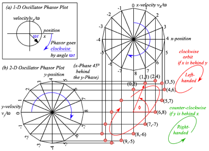
Fig. 9.10 Oscillator plots. (a) 1D-HO phasor plot. (b) Isotropic 2D-oscillator phasors and xy-path.
First we verify by algebra that orbits in Fig. 9.10 and Fig. 9.11 are ellipses. Fig. 9.11a has x running 90° behind y with a relative phase lag Äá=áx−áy=ð/2 that is 4 hours or 1/4-period behind in phase on a 16-hour clock. We say such a 90°-lagging-x-motion is in-quadrature to y-motion. It gives an un-tilted ellipse with a left-handed orbit, and if ex=a=b=ey then it gives a circular orbit or left-circular polarization. (See Fig. 9.11a on right.) For right-handed orbits x-motion and x-motion switch leads to Äá=áx−áy=−ð/2.
In-quadrature xy -motion is a cosine and sine projection on a-side and b-side of an ellipse, respectively, based on expressions (9.8).
x = a cos ù t , (9.13a) y = b cos(π/2-ù t) = b sin ù t . (9.13b)
Squaring and adding cosine and sine expressions gives a standard xy-ellipse equation.
![]() (9.13c)
(9.13c)
Zero phase lag Äá =0 or in-phase motion gives linear polarization in Fig. 9.11b. In the case of Fig. 9.11b where x and y-motions are in-phase we have
x = a cos ù·t , (9.14a) y = b cos ù·t . (9.14b)
Combining these two gives a trajectory that follows a straight line of slope (b/a) seen in the figure.
y = (b/a) x (9.14c)
Lag Äá =±ð or pi-out-of-phase is a linear polarized motion, too.
x = a cos ù·t , (9.15a) y = -b cos ù·t . (9.15b)
It is simply a horizontal mirror reflection of the in-phase path.
y =-(b/a) x (9.15c)
In each of the figures we could imagine three starlets going in unison. The first starlet obeys the y-equation (9.13b) with x=0. The second starlet obeys the x-equation (9.13a) with y=0 and tunnels as in Fig. 9.8. A third starlet obeys both the x and y equations like the starlet orbiting above the tunneling one(s).
In a linear force field F=-kr all Cartesian components oscillate sinusoidally at the same frequency.
F=-kr implies : Fx=-kx , Fy=-ky , Fz=-kz (9.15)
Neither the coulomb field F=-kr/r3 nor any other power-law field F=-krrp is so convenient!
As shown in Unit 5, negative energy orbits in Coulomb fields are also elliptic, and elegant ruler & compass geometry gives them, too. However, Coulomb ellipses are symmetric about origin only for circular orbits. All other Coulomb orbits are eccentric since they orbit about an off-center focal point and not the ellipse center of symmetry that lies at origin (r=0) for any Hooke’s law oscillator orbit of a starlet.
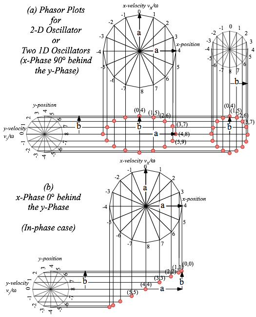
Fig. 9.11 Two 1-D oscillator phasor plots combine to give 2D-oscillator xy-trajectory.
Exercise 1.9.3. Tunnels to UK (5600 miles away as an earthworm crawls) are shown below. One high-road is a direct route. The other low-road turns around at the Earth center. Travel and turn-around are assumed frictionless and survivable. (a) How long is each trip? Discuss.
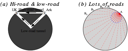
(b) A network of subways leaving Ark. at time t=0. What curve (like the dots) describe each moment?
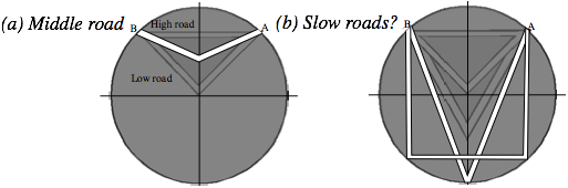
Exercise 1.9.4. Consider competing tunnels between points A-to-B separated by R√2~ 5600 miles (thru Earth) or Äö=90° of longitude and 6 Time Zones. The preceding problem asked you to compare the high-road or direct-route to the low-road or via-Earth-center-and-back-route. Here we consider middle-road routes such as in Fig (a) below. (a) Find the fastest 2-straight-section middle road A-to-B by geometry or algebra. How much faster is it? (Give answer for local travel:Äö=1°, long distance:Äö=90° and for general Äö.)
(b) How long does it take to go from A-to-B on slow-roads (“V”-road and “U”-road) in Fig. (b).
Exercise 1.9.5. Construct 24-point neutron-starlet orbits (One point for every hour assuming a 24-hour orbital period.) inside a uniform asteroid with x-component oscillation amplitude exactly equal to that of y and the x-component phase fixed relative to that of y as follows:
(a) x is in phase with y. (b) x is behind y by 1 hour. (c) 2 hours. (d) 3 hours. (e) 4 hours. (f) 5 hours. (g) 6 hours. (h) 7 hours.
Do the orbits change if we replace behind by ahead in (a) to (h)? Discuss or describe.
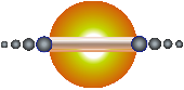 (Scale of
ball-towers greatly magnified)
(Scale of
ball-towers greatly magnified)
Super-Duper-Nova Model
1.9.6 Identical ball towers are dropped toward each other from opposite sides of Earth into a center-of-Earth tunnel. How many can bounce back up to surface and how many of those reach escape velocity for:
(a) N=2 case: m2 = 1, m1=2. (b) N=4 case: m4 = 1, m3=2, m2=4, m1=8.
Chapter 10 Calculus of exponentials, logarithms, and complex fields
A logarithmic potential curve U=ln(y)=logey was given by (6.11). Our first example is the flip or inverse exponential curve y=eU since that function is so important for making the complex phasor e-(iù+Ã)t.
Also, the population growth function y=et=exp(t) is one of the most used if not the most useful of transcendental functions. Roughly, transcendental means not expressed by finite algebra or constructed by Euclid’s strict rules. (However, like transcendental spirituality, it is easily approximated!) Later in this section we will prove that the exponential is the only function that is equal to its slope or derivative.
![]() (10.1)
(10.1)
In other words, if ex is a force or potential curve then F(x) and U(x) are similar, in fact, identical.
Fmath(x) ![]() = U(x). if and only if: U(x)=ex (10.2a)
= U(x). if and only if: U(x)=ex (10.2a)
For physicist’s definition (6.9) of force, e-x is the one for which potential and force are identical.
Fphys(x)
![]() = U(x). if and only if: U(x)= e-x (10.2b)
= U(x). if and only if: U(x)= e-x (10.2b)
For now we use these slope-function relations to construct the exponential curve approximately. Starting from origin (x=0) we use the fact that any positive number to zero power is 1. (e0=1) From that point we draw a right triangle made of a unit altitude, a unit base, and a hypotenuse line of slope-1 as indicated in Step-0 of Fig. 9.12. The hypotenuse line gives approximately the points just above and just below x=0. Then subsequent steps move the right triangle Äx to a point on the previously constructed line to make the next line. Since the slope is equal to the new function value, the base stays fixed at 1, but the altitude grows with the function value and makes the new line and a new point up the ex-curve.
This approximation is a rough one. It underestimates a concave curve and overestimates convex ones because it puts the next point x+Äx on a tangent from the previous point x. That’s OK only if the curve is pretty straight and tangent slope is about the same at x+Äx. A better approximation uses the tangent halfway between neighboring tangents and extends that new slope to x+Äx to find the next point.
Now if you rotate your y= ex-graph by 90° you get a logarithm U(y)=-ln(y) graph as shown in Fig. 10.1 (lower right). Each U(y)-curve-normal defines a unit-altitude triangle whose base is the force F(y)=1/y.
The story of e : A tale of great interest
Long ago banks would pay simple interest at some rate r such as r=0.03 (3%) based on a 1 year period. You gave a principal p(0) to the bank and some time t later they would pay you p(t)=(1+r·t)p(0). If you put in $1.00 at rate r=1 (like Israel and Brazil that once had 100% intrest.) you got $2.00 at t=1year.
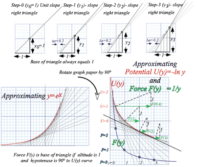
Fig. 10.1 Rough constructions (a) exponential curve y=ex=exp(x). (b) Log potential. (c) 1/y-Force.
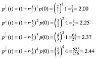
Later on fancy banks would pay semester compounded interest ![]() at the
half-period
at the
half-period ![]() and then use
and then use ![]() during
the last half to figure final payment. Now $1.00 at rate r=1 earns $2.25.
during
the last half to figure final payment. Now $1.00 at rate r=1 earns $2.25.
![]()
Fancier banks would pay trimester compounded interest ![]() at
the 1/3rd-period
at
the 1/3rd-period ![]() or 1st trimester and
then use that to figure the 2nd trimester and so on. Now $1.00 at
rate r=1 earns $2.37.
or 1st trimester and
then use that to figure the 2nd trimester and so on. Now $1.00 at
rate r=1 earns $2.37.
![]()
Still fancier banks would pay quarterly, monthly, weekly, daily, and so on. The race was on to give better earnings at a given interest rate r. Let’s compare some different earnings on $1.00 at rate r=1. At first it looks like you gain a lot by compounding more often. Then earnings slow to a halt just shy of $2.72.

That halting
point is Euler’s
growth constant e=2.718281828459… that we’re after. Let's try huge
numbers (m)
of multiplications in ![]() .
(Get out a calculator. Rule & compass is useless now!)
.
(Get out a calculator. Rule & compass is useless now!)
p1/m(1) = 2.7169239322 for m = 1,000
p1/m(1) = 2.7181459268 for m = 10,000
p1/m(1) = 2.7182682372 for m = 100,000
p1/m(1) = 2.7182804693 for m = 1,000,000 (10.3)
p1/m(1) = 2.7182816925 for m = 10,000,000
p1/m(1) = 2.7182818149 for m = 100,000,000
p1/m(1) = 2.7182818271 for m = 1,000,000,000
The solid figures represent numbers that stay the same as we raise m. It’s still a torturous way to find e. We do a Billion (That’s “B” as in “Boy!”) multiplications (m=109) just to get 6 solid figures beyond 2.71.
A
better way expands binomial ![]() or
its power
or
its power ![]() for
all rates r and times t.
We let mr·t=n and m =n/r·t to simplify it for huge multiplication numbers m or n.
for
all rates r and times t.
We let mr·t=n and m =n/r·t to simplify it for huge multiplication numbers m or n.
![]() (10.4)
(10.4)
A binomial expansion
(See
page 119) turns exponential
function er·t into a power series in ![]() with x=1.
with x=1.
![]()
We actually save work as multiplication number n gets huge! (“Huge” means “as close to ∞ as you like.”)
![]()
Huge n makes n(n-1) cancel n2 , and n(n-1)(n-2) cancel n3 , and so on. The exponential er·t series is born.
![]() (10.5a)
(10.5a) ![]() (10.5b)
(10.5b)
Let’s try it out for r·t=1 to evaluate e to order-o. (The precision order o is the power of highest term used.)
Precision order: (o=1)-e-series = 2.00000 =1+1
(o=2)-e-series = 2.50000 =1+1+1/2
(o=3)-e-series = 2.66667 =1+1+1/2+1/6
(o=4)-e-series = 2.70833 =1+1+1/2+1/6+1/24
(o=5)-e-series = 2.71667 =1+1+1/2+1/6+1/24+1/120 (10.6)
(o=6)-e-series = 2.71805 =1+1+1/2+1/6+1/24+1/120+1/720
(o=7)-e-series = 2.71825
(o=8)-e-series = 2.71828
Nine terms in series (10.5) give 5-figure accuracy (10.6) and do the work of a million products in (10.3). That’s a million reduced to 8 sums and half-dozen or so divisions. It’s a big savings of arithmetic labor!
Derivatives, rates, and rate equations
Binomial expansions provide ways to find calculus formulas for slope or velocity introduced geometrically in Ch. 1. Soon we will do the same for curvature or acceleration and other higher order calculus concepts.
Suppose someone gives you a plot of formula like x(t)=t2 or x(t)=sin4t or an exponential plot of x(t)=et that we just did in Fig. 10.1. You should be able to estimate its slope at any point from its x versus t graph. However, a binomial expansion may let you find an exact formula for its slope.
Consider a parabola x(t)=t2 for example. Let’s find the slope ![]() of a line
that goes through point x(t) and a point x(t+Ät) =(t+Ät)2 that is a tiny time interval Ät later. Binomial expansion gives Äx=x(t+Ät)-x(t).
of a line
that goes through point x(t) and a point x(t+Ät) =(t+Ät)2 that is a tiny time interval Ät later. Binomial expansion gives Äx=x(t+Ät)-x(t).
Äx=x(t+Ät)-x(t)=(t+Ät)2-t2=t2+2t·Ät+(Ät)2-t2=2t·Ät+(Ät)2
Slope ratio![]() follows. If Ät is
tiny we ignore it. Then tangent slope
follows. If Ät is
tiny we ignore it. Then tangent slope ![]() is the
1st
derivative of x(t)=t2.
is the
1st
derivative of x(t)=t2.
![]() (10.7a)
(10.7a) ![]() (10.7b)
(10.7b)
This checks the geometry of parabola 2ëy=x2 in Fig. 9.4. Slope is ![]() , twice the x-value in units of 2ë. Consider an n-power
curve x(t)=Atn. Binomial expansion of Äx=x(t+Ät)-x(t) has n
terms, most in +…+.
, twice the x-value in units of 2ë. Consider an n-power
curve x(t)=Atn. Binomial expansion of Äx=x(t+Ät)-x(t) has n
terms, most in +…+.
Äx=x(t+Ät)-x(t)=A(t+Ät)n-Atn=Atn+Antn-1·Ät+…+A(Ät)n-Atn=Antn-1·Ät+…+A(Ät)n
If Ät
is tiny, only 1st
term Antn-1 in slope ratio![]() is not tiny-tiny. That 1st term is 1st derivative of x(t)=Atn.
is not tiny-tiny. That 1st term is 1st derivative of x(t)=Atn.
![]() (10.8a)
(10.8a) ![]() (10.8b)
(10.8b)
Series for x(t)=Aet is unchanged (for r=1) by ![]() . It does
kill term number-∞, but
. It does
kill term number-∞, but ![]() is tiny-tiny-tiny anyway.
is tiny-tiny-tiny anyway.
 (10.9)
For 100% intrest (r=1), growth rate-of-Aet equals Aet. Otherwise, growth rate of Aert is proportional to Aert. To state that the growth rate of a function x(t) equals a constant “intrest rate” r times current value of x(t) is to write a differential rate equation whose “solution” is x(t)=Aert. (The constant A is “initial capital” A=x(0).)
![]() (10.10)
(10.10)
It is Malthus’s population explosion equation for positive rate r>0! It is radioactive decay equation for r<0.
High school algebra courses generally contain a treatment of the binomial theorem that is used for our er·t expansion after equation (10.4). In case your course missed that (or you weren’t paying attention!) we’ll take a close look at this remarkable formula. The binomial algebra and related Pascal triangle geometry is the basis of so much mathematics and physics that it deserves a book chapter of its own.
First
it helps to work out the first few binomial series (x+y)0,
(x+y)1, ![]() (x+y)2,
(x+y)3,… by
simply multiplying them together as we did for the er·t series that started this discussion. The
first examples (x+y)0=1 and (x+y)1=x+y are easy since the 0th and 1st powers of a number n are defined to be 1 and n,
respectively. The square of a binomial is simple enough, too.
(x+y)2,
(x+y)3,… by
simply multiplying them together as we did for the er·t series that started this discussion. The
first examples (x+y)0=1 and (x+y)1=x+y are easy since the 0th and 1st powers of a number n are defined to be 1 and n,
respectively. The square of a binomial is simple enough, too.
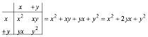
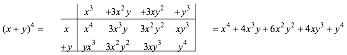
(x+y)2=(x+y)·(x+y)=x2+xy+yx+y2= x2+2xy +y2 (1)
You might find it helps to make a table of product terms to do algebraic multiplication of this sort. Just make a box and write one factor ((x+y) in this case) on top and the other ((x+y) again) along the left.
![]()
 (2)
(2)
The just multiply each thing on top by each thing on the left and add them up to get (1). Try it with (x+y)3.
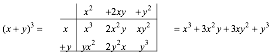 (3)
(3)
We can continue this process to get (x+y)4, (x+y)5,…and so forth.
 (4)
(4)
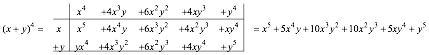 (5)
(5)
After awhile, you might notice a pattern in the numbers or coefficients Bpq of the various power terms xpyq where the powers p and q must add up to the power n=p+q of (x+y)n being calculated. These Bpq are called the binomial coefficients of xpyq and a triangular array pattern in Fig. 1 is called Pascal’s triangle.
This pattern is like a Ponzi scheme since every number in it except the pinnacle B00=1 is the sum of one or two numbers that lie above it and to either side. (This sum is going on in (2) thru (5) above.) So the pinnacle position q-p=0 on the central vertical triangle axis ends up with the biggest number Bpq for each power-row n=p+q. At n=p+q =10th row, pinnacle B5,5 accumulates 252 from 11 spots –5<q-p<+5.
Table 1. Binomial combinatorial coefficients up to power n=10
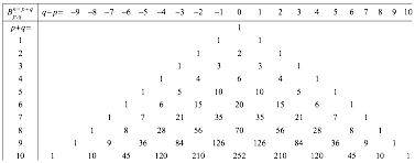
Gamblers may recognize B55=252 as the number of ways you can get exactly 5 x-cards and 5 y-cards from an n=20 card deck of 10 x-cards and 10 y-cards. More simply, B55=252 is the number of ways to get exactly 5 heads and 5 tails from an n=10 coin tosses, or x5y5 from an (n=10)-power binomial.
(x+y)(x+y)(x+y)(x+y)(x+y)(x+y)(x+y)(x+y)(x+y)(x+y)=(x+y)10=x10+…252x5y5+…y10 (7)
As you go down the line of 10 factors (x+y) you must pick x or y from each factor (x+y) to make just one (n=10)-power term xpyq with n=p+q. There are 210 =1024 such terms. (Just add up the 10th row of Table 1.)
(1+1)10=210=110+…252·1515+…=1+10+45+120+210+252+210+120+45+10+1=1024 (8)
Check the other rows, too. (It’s a good to know powers-of-2 in a binary age!)
22=4, 23=8, 24=16, 25=32, 26=64, 27=128, 28=256, 29=512, 210=1024,… (9)
Now suppose, instead of just two things x or y, you could choose n different things {a,b,c,…,x,y,z,..} from each of the n factors in (7). Then the number of ways you may get a given term a·b·c·…·x·y·z·.. having all n different things is the number n!=n·(n-1)·(n-2)·…·2·1 of permutations of n things. Each permutational reordering gives another equal term (a·b=b·a).
So, n! is the “n-nomial coefficient” for a term with n-different factors. However, if we are counting terms xpyq like a binomial series has with only two different things, the p! permutations of the x things and the q! permutations of the y things do not count as new terms. Then n! divided by p! and q! gives Bpq.
![]() examples:
examples: ![]()
This
gives binomial series that follows (10.4) and the Gauss-binomial distribution
plotted below.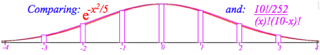
General power series approximations
Are power series like (10.5) useful for functions other than exponentials? Well, Mr. Maclaurin and Mr. Taylor thought so. Series that bear their names are de rigeur in good math books. (And, in this one, too!)
Let’s start with a general power series like (10.5) but with arbitrary constant coefficients c0, c1, etc.
![]() (10.11a)
(10.11a)
We derive c0 by setting time t to an initial time t=0. (Like C-programmers, we count “uh-zero, uh-one, uh-two,..”)
c0 = x(0) (10.11b)
So the 0th coefficient c0 is initial position x(0). Now we use (10.8b) to find a derivative of each term.
![]() (10.11c)
(10.11c)
Rate of change of position x(t) is velocity v(t). Setting t=0 derives c1.
c1 = v(0) (10.11d)
So the 1st coefficient c1 is initial velocity v(0). Now find a 2nd derivative using (10.8b).
![]() (10.11c)
(10.11c)
Change of velocity v(t) is acceleration a(t). Set t=0 to get c2.
c2 = ![]() a(0) (10.11d)
a(0) (10.11d)
So the 2nd coefficient c2 is half the initial acceleration a(0). Now a 3rd derivative:
![]() (10.11e)
(10.11e)
Change of acceleration a(t) is jerk j(t). (Jerk is a NASA sanctioned term!) Set t=0 to get c3.
c3 =![]() j(0) (10.11f)
j(0) (10.11f)
So the 3rd coefficient c3 is initial jerk j(0) over 3! Now a 4th derivative:
![]() (10.11g)
(10.11g)
Change of jerk j(t) is inauguration i(t). (If NASA can be silly, so can we!) Set t=0 to get c4.
c4 =![]() i(0) (10.11h)
i(0) (10.11h)
So the 4th coefficient c4 is initial inauguration i(0) over 4!. Now a 5th derivative.
![]() (10.11i)
(10.11i)
Change of inauguration i(t) is revolution r(t). (Ooops! Politically incorrect!) Quick set t=0 to get c5.
c5 =![]() r(0) (10.11j)
r(0) (10.11j)
That’s enough iterations to show the Maclaurin series of any function x(t) that has decent derivatives.
![]() … (10.12a)
… (10.12a)
By “decent” we mean the non-exploding types that we can deal with. The following is a list that shows some of the notations used for the higher order derivatives discussed so far.
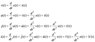 (10.12b)
The “dot” notation writes n-derivatives of x(t) by puttting n-dots over x. This may help prevent writer’s cramp.
But, j-dot looks, well, kind of jerky. It’s common
to use primes (![]() )
for x-derivatives.
)
for x-derivatives.
How good is a power series (10.5) at faking x=et beyond t=1listed in (10.6)? We plot various orders of approximation in Fig. 10.2. The 1st order (2-terms of (10.5a)) is just a straight line of slope 1. A 2nd order (3-term) parabola, 3rd order cubic, 4th order quartic, etc. each peel off x=et in sucession. All meet at (t=0,x=1).
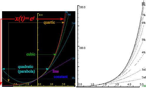
Fig. 10.2 Comparing x=et with its nth-order approximate power series.
A severe test of power series is their ability to fake sine waves. The derivative and rate equation for the sine function x(t)=sinùt uses expansion x(t+Ät)=sinù(t+Ät). To expand sin(a+b) or cos(a+b) we use Fig. 10.3.
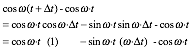
sin(a+b)= cosa sinb + sina cosb (10.13a) cos(a+b)= cosa cosb - sina sinb (10.13b)
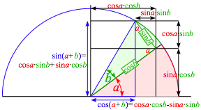
Fig. 10.3 Geometry of sine and cosine expansion identities.
Expansion of Äx=x(t+Ät)-x(t) for sine or cosine is easy since sinù·Ät=ù·Ät and cosù·Ät=1 for tiny Ät.
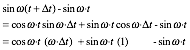
![]() (10.14a)
(10.14a) ![]() (10.14b)
(10.14b)
We will need the sine and cosine slope (derivative) formulas that follow from this.
![]()
![]()
![]() (10.15a)
(10.15a) ![]() (10.15b)
(10.15b)
A list of series coefficients![]() in (10.12)
for sine x=sin
ùt and cosine x=cos ùt is worked out below.
in (10.12)
for sine x=sin
ùt and cosine x=cos ùt is worked out below.
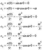
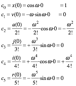
A sine derivative repeats after four orders: …sin t, cos t, -sin t, -cos t, (again) sin t, cos t, -sin t, -cos t, (etc.) .
The resulting sine and cosine series show
this repeat-after-4-pattern of factors 0,1,0,-1 of ![]() terms.
terms.
![]()
![]()
(10.16a) (10.16b)
The sine is an odd function to time reversal (sin(-t) =-sin(t)), but cosine is even (cos(-t)
=+cos(t)). Thus sine has
only odd powers p=1,3,5,… of time and cosine has only even powers p=0,2,4,…. Series plots (10.16) in Fig. 10.4 have
highest power or order o=1st,2nd,3rd,4th,etc. Number n of terms is ![]() for
sine and
for
sine and ![]() for
cosine.
for
cosine.
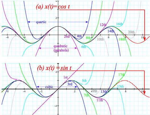
Fig. 10.4 Comparing (a) x=sin t and (b) x=cos t with their nth-order approximate power series.
It takes a 9th (for sin t) or 10th (for cos t) order series of 5 terms to get one full oscillation with 5% or better precision. Then 10 terms gives two oscillations, and so on. Fig. 10.4 shows that precision breaks down quite explosively. Polynomials are exponentially degrading approximations of wave motion.
Sine, cosine, and ert power series (10.16) and (10.9) lead to an 18th Century crown jewel of mathematics. It is due to a close relation of these series and the functions they represent. It is hard to imagine, but exponential intrest rate growth and simple harmonic oscillation are related. As it turns out, the relation is quite imaginary!
Suppose
the fancy bankers really went bonkers and made intrest rate r an imaginary number
r=iè. Imaginary number ![]() has
powers with a repeat-after-4-pattern: i0=1,
i1=i, i2=-1, i3=-i, i4=1,etc... It fits the pattern leading to cosè and sinè series (10.16). Series (10.9) with imaginary rt=iè joins the (10.16) series.
has
powers with a repeat-after-4-pattern: i0=1,
i1=i, i2=-1, i3=-i, i4=1,etc... It fits the pattern leading to cosè and sinè series (10.16). Series (10.9) with imaginary rt=iè joins the (10.16) series.
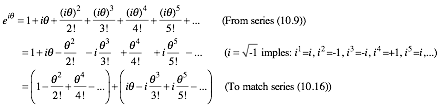
![]() (10.17)
(10.17)
The resulting Euler-DeMoivre
Theorem is a beautiful
identity and a very powerful tool as we shall see. First and foremost it is a complex wave phasor
function ![]() that we will use in Unit 4. (Note: è =-ù·t.)
that we will use in Unit 4. (Note: è =-ù·t.)
![]() (10.18)
(10.18)
Fig. 10.5a plots ![]() in the complex plane, a real-vs-imaginary graph. Fig. 10.5b shows
in the complex plane, a real-vs-imaginary graph. Fig. 10.5b shows![]() as a complex phasor clock. Real part
Reø =x(t) is position. Imaginary part is ù-scaled
velocity Imø =v(t)/ù. Conversion of polar-to-Cartesian (10.19a) and vice-versa (10.19b) is on scientific calculators. (Recall cautions
at end of Ch. 1.)
as a complex phasor clock. Real part
Reø =x(t) is position. Imaginary part is ù-scaled
velocity Imø =v(t)/ù. Conversion of polar-to-Cartesian (10.19a) and vice-versa (10.19b) is on scientific calculators. (Recall cautions
at end of Ch. 1.)
![]() (10.19a)
(10.19a) ![]() (10.19b)
(10.19b)
Real part Reø is the
“is” (that Clinton sought in 1997) and Imø is
what Reø is “gonna-be” in![]() -cycle (as in “gonna be
in trouble!” A mantra,“Imagination
precedes reality by one quarter”
works here as in US corporate world.) Euler expo-sinusoidal identities relate cosè, sinè, and e±iè. A conjugate ø* reflects i with –i.
-cycle (as in “gonna be
in trouble!” A mantra,“Imagination
precedes reality by one quarter”
works here as in US corporate world.) Euler expo-sinusoidal identities relate cosè, sinè, and e±iè. A conjugate ø* reflects i with –i.
![]() (10.20a)
(10.20a)
![]() (10.20b)
(10.20b)
A special case is e-iπ=-1. (We’ll also use a real π-exponential: e-π=0.04321.) Other special cases are noted.
![]() ,
, ![]() ,
, ![]() . (10.21)
. (10.21)
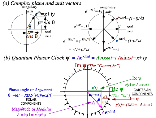
Fig. 10.5 (a) Complex plane. (b) Phasor clock. Cartesian form uses (Reø, Im ø). Polar form uses (|ø|,è).
Wages of imaginary intrest: Phasor oscillation dynamics
By now bankers should know what happens when you use imaginary intrest. The accounts oscillate up and down and the imagineering bankers oscillate in and out of the slammer. (At least that was the way until 2001 when the Bush administration passed the No Banker Left on His Behind Act that also outlawed reality.)
Consider exponential rate equation (10.15) with negative imaginary rate r=-iù.
![]() (10.22a)
(10.22a)
It becomes a real 2nd order equation if we apply the derivative operation to both sides.
![]() (10.22b)
(10.22b)
It is the Newton-Hooke simple harmonic oscillator equation, but it has the same solution as (10.19) above.
![]() (10.23a)
(10.23a)
It combines Newton’s force law F=m·a=m![]() and Hooke’s force law F=-k·x. The ù value
repeats (9.9b).
and Hooke’s force law F=-k·x. The ù value
repeats (9.9b).
![]() (10.23b)
(10.23b)
What Good Are Complex Exponentials?
Complex Exponentials are used to describe oscillation, resonance, waves and fields. We don't use them just to be cute! Let’s look at some compelling reasons for using imaginary or complex arithmetic.
Complex numbers provide "automatic trigonometry"
If you have trouble remembering trigonometric identities then this is a good reason all by itself to use complex numbers. For example, if you're taking a test and you can't remember what is cos(a+b), then just factor ei(a+b) = eiaeib, expand exponentials into eia = cos a + i sin a and multiply them out.
ei(a+b) = eiaeib
cos(a+b) + i sin(a+b) = (cos a + i sin a) (cos b + i sin b)
cos(a+b) + i sin(a+b) = [cos a cos b - sin a sin b]+i[sin a cos b + cos a sin b] (10.24a)
That’s two trig identities for the price of one! The real part gives the cosine relation (10.13b).
cos(a+b) = [cos a cos b - sin a sin b] (10.24b)
The imaginary part gives the sine relation (10.13a).
sin(a+b) = [sin a cos b + cos a sin b]. (10.24c)
Complex exponentials Ae-iùt tracks position and velocity using Phasor Clock.
Recall discussion of phasor diagram in Fig. 10.5b. Real and imaginary give phase: position and velocity.
Complex numbers add like vectors.
Physics of wave interference involves the addition or subtraction of oscillating signals. If the signals are represented by complex numbers then you simply add (or subtract) their Cartesian components.
zsum = z + z' = (x + iy) + (x' + iy') = (x + x') + i(y + y')
zdiff = z − z' = (x + iy) − (x' + iy') = (x − x') + i(y − y')
Before adding, convert z and z' to Cartesian (x,y) form if given in polar form z=reiö and z'=r'eiö'. Radius r of a vector z is its magnitude or complex absolute value |z|. Square |z|2 is proportional to energy or intensity.
|z| = r = √(x2 + y2) = √([x - iy][x + iy]) = √(z*z)
We write |z|2 as product of z and its complex conjugate z* = x - iy =re-iö to derive radius |zsum| of a vector sum zsum or radius |zdiff| of a difference zdiff. It is an easy way to get the well-known cosine laws.
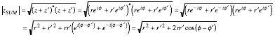 (10.25a)
![]() (10.25b)
(10.25b)
Vector diagrams of sum, difference, and product of complex z and z′ are shown in Fig. 10.6.
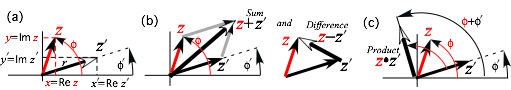
Fig. 10.6 Parallelogram diagonals are sum zsum=z+z' and difference zdiff=z-z' vectors.
Complex products provide 2D rotation operations.
A product zz' of two complex numbers expressed in Cartesian form as z = x + iy and z'= x'+ iy' is
z z' = (x + iy) (x' + iy') = [xx' - yy'] + i[xy' + yx'].
It is simpler if the numbers are expressed in polar form as z = r eiö and z' = r' eiö'.
z z' = ( reiö )( r'eiö' ) = r r' ei(ö+ö'). (10.26)
Note that multiplication results in addition of exponents and a sum of polar angles. Radii multiply to give a product rr' but angles add to give a sum (ö + ö'). You might imagine z rotating vector z' by ö radians or that z' rotates z by ö' radians. Consider in detail a rotational operator eiö on a vector z =(x + iy).
eiö·z = (cosö + i sinö)·(x + iy)= x cosö − y sinö + i(x sinö + y cosö ) (10.27a)
Ch. 5 2-by-2 rotation matrix Rö (Fig. 5.3d) acts on a 2D vector r to give results precisely similar to eiö·z.
![]() (10.27b)
(10.27b)
![]() (10.27c)
(10.27c)
Complex products set initial values
Phase angle -ùt of phasor e-iùt rotates clockwise with time. Multiplying e-iùt by a complex amplitude A =|A|eiñ sets its phase back by angle ñ and its radius to |A|. Amplitude A is the initial value x(0)=|A|eiñ.
x(t)=Ae-iùt = x(0)e-iùt = |A|eiñe-iùt = |A|e-i(ùt-ñ) (10.28)
Such products set initial values of oscillator clocks. A positive angle ñ is a phase lag since it moves the phasor counter-clockwise and sets its clock back. A negative angle ñ=−|ñ| gives a phase lead.
Complex products provide 2D “dot”(•) and “cross”(x) products.
Consider any two vectors A=Ax+iAy and B=Bx+iBy and their “star” (*)-product A*B.
![]() (10.29)
(10.29)
Real part is scalar or “dot”(•) product A•B. Imaginary part is vector or “cross”(×) product, but just the Z-component normal to xy-plane. To better understand this math trickery, we rewrite A*B in polar form.
![]() (10.30a)
(10.30a)
This matches standard 3D definitions of dot(•) and cross(×) products in Appendix 1.A of this Unit.
![]()
![]() (10.30b)
(10.30b)
Expansion (10.24) of Ä-angle ![]() relates
reiè forms (10.30) to xy-forms in (10.29).
relates
reiè forms (10.30) to xy-forms in (10.29).
![]()
![]()
![]() (10.30c)
(10.30c) ![]() (10.30d)
(10.30d)
Complex deriviative contains “divergence”(∇•F) and “curl”( ∇xF) of 2D vector field
By
relating (z,z*) to (x=Rez,y=Imz) we may define a z-derivative![]() and “star” z*-derivative
and “star” z*-derivative![]() .
.
![]()
![]()
![]() (10.31)
(10.31)
Derivative chain-rule shows real part of ![]() has 2D
divergence ∇•F
and imaginary part has curl ∇×F.
has 2D
divergence ∇•F
and imaginary part has curl ∇×F.
![]() (10.32)
(10.32)
Now we can invent source-free 2D
vector fields that are both
zero-divergence and zero-curl by taking any function f(z) and conjugating it (change all i’s to –i) to give f*(z*) for which ![]() . For
example, if f(z)=a·z then f*(z*)=a·z*=a(x-iy) is not a function of z
so it has zero z-derivative, hence zero ∇•F and zero |∇×F|.
. For
example, if f(z)=a·z then f*(z*)=a·z*=a(x-iy) is not a function of z
so it has zero z-derivative, hence zero ∇•F and zero |∇×F|.
F=(Fx,Fy)=(f*x,f*y)=(a·x,-a·y) has zero divergence: ∇•F=0 and has zero curl: |∇×F|=0. (10.32)
A plot of vector field F=(f*x,f*y) =(a·x,-a·y) in Fig. 10.7 shows a divergence-free laminar (DFL) flow field.
Complex potential ö contains “scalar”( F= ∇Ö) and “vector”( F=∇xA) potentials
Any DFL flow field F is a gradient of a scalar potential field Ö or a curl of a vector potential field A.
F= ∇Ö F= ∇×A
There is a complex potential ö(z)=Ö(x,y)+iA(x,y) whose z-derivative is f(z) and it comes with its complex conjugate ö*(z*)=Ö(x,y)-iA(x,y) whose z*-derivative is the f*(z*) that we use to plot DFL flow fields F.
![]() (10.33a)
(10.33a) ![]() (10.33b)
(10.33b)
Derivative ![]() by
(10.31) has 2D gradient
by
(10.31) has 2D gradient ![]() of
scalar Ö and curl
of
scalar Ö and curl ![]() of vector A.
of vector A.
![]() (10.34)
(10.34)
Some more math trickery has “vector-A” be just a “Z-component” A=Azez normal to the complex (x,y)-plane. So A(x,y)=Az(x,y) is treated as a single function of (x,y) like scalar Ö(x,y). Also, a mathematician definition for force field F=+∇Ö replaces our usual physicist’s definition F=-∇Ö of (6.9). (No annoying (-)-sign now!)
To find ö=Ö+iA we integrate f(z)=a·z to get ö and isolate real (Reö=Ö) and imaginary (Imö=A) parts.
![]() (10.35a)
(10.35a)
Note: either
part gives the whole F field. Factors ![]() in (10.34)
could be
in (10.34)
could be ![]() or
or![]() or any (f,j) with f+j=1.
or any (f,j) with f+j=1.
![]() (10.35b)
(10.35b) ![]() (10.35c)
(10.35c)
Scalar static potential lines Ö=const.
and vector flux
potential lines A=const. define a field-net in
Fig.10.7.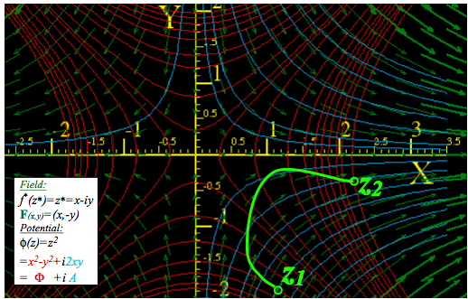
Fig.10.7 Complex field f(z)=z of F=(x,-y) vectors on potentials of static Ö=(x2-y2)/2 and flux A=xy.
Complex integrals ∫ f(z)dz count “flux”( ∫Fxdr) and “vorticity”( ∫F•dr)
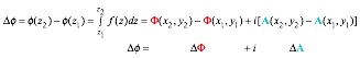
Integral f(z) (10.35a) between point z1 and point z2 in Fig. 10.8 is potential difference Äö=ö(z2)- ö(z1) between the end-points. In DFL fields, Äö is independent of the integration path z(t) connecting z1 and z2.
 (10.36)
The real part ÄÖ
of Äö is work ![]() done
pushing r up a hill in Fig. 10.8. (Now force F= ∇Ö points
up-slope.) Since F=(f*x,
f*y)
is plotted using f*(z*), we set f(z)=(f*(z*))* to get real and imaginary parts of f(z)dz.
done
pushing r up a hill in Fig. 10.8. (Now force F= ∇Ö points
up-slope.) Since F=(f*x,
f*y)
is plotted using f*(z*), we set f(z)=(f*(z*))* to get real and imaginary parts of f(z)dz.
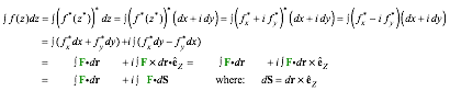 (10.37)
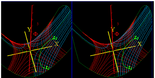
Fig. 10.8 Stereo-3D view of Fig. 10.7(ö(z)=z2/2) plots static potential Ö normal to xy-axes.
Real part ![]() sums F projections along path vectors dr to get ÄÖ in
(10.36). Imaginary part
sums F projections along path vectors dr to get ÄÖ in
(10.36). Imaginary part ![]() sums
F projection across dr
that is, it sums flux thru surface elements dS=dr× normal to dr to get ÄA.
sums
F projection across dr
that is, it sums flux thru surface elements dS=dr× normal to dr to get ÄA.
One
power-law field f(z)=azn lacks a power-law potential![]() . It is
. It is ![]() . Its
integral is a logarithmic potential
ö(z)=a·ln(z)=a·ln(x+iy). (Recall (6.11).) Use ln(a·b)=ln(a)+ln(b), ln(eiè)=iè, and z=reiè.
. Its
integral is a logarithmic potential
ö(z)=a·ln(z)=a·ln(x+iy). (Recall (6.11).) Use ln(a·b)=ln(a)+ln(b), ln(eiè)=iè, and z=reiè.
![]() (10.38)
(10.38)
Potential a·ln(z) is the field of a line of charge q if a=q is real and a line of current J if a=iJ is imaginary. Fig. 10.9a is a diverging F-field of unit charge (q=1) and Fig. 10.9b is a curling F-field of unit current (J=1). Line charge F-field is like an electric E-field. Line current F-field is like a magnetic B-field of a wire, a vortex.
F-field and radial streamlines (A=è =const.) diverge normal to equal-Ö circles (Ö=r =const.) in Fig. a. F-field and circular streamlines (A=r =const.) curl clockwise normal to radial equal-Ö lines (Ö=è =const.) in Fig. b. (The clockwise (-i)-sense of rotation results from plotting f*(z*)=-i/z* as our (*)-convention requires.)
Stereo-3D potential plots of real-line-source field shown in Fig. 10.10a show mathematical structure of its Ö and A potentials that lets us compare them to imaginary-line-source potentials in Fig. 10.10b. Real part Ö=ln(r) of (10.38) for real (a=1)-source in Fig10.10a is a surface like a morning-glory. Blue-(A=è=const.) -streamlines stream down its throat normal to (Ö=r =const.) level circles.
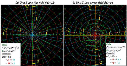
Fig. 10.9 Fields due to a unit Z-line-source normal to center. (a) Real source a=q=1. (b) Imaginary a=iJ=i.
Below that Ö-vs-(x,y)-plot is a 3D A-vs-(x,y)-plot for the same real source in Fig. 10.10a. Imaginary part A=è of (10.38) gives radial steps that are level lines of a single helix or helicoid. Red-(Ö=r =const.)-lines stream up its spiral staircase normal to (A=è=const.) steps. At the top step A=è=π , above the –X-axis, is a “waterfall” of red lines falling by ÄA=2π straight to bottom helical step A=è=-π. This 2πi-fall of complex potential ö(z) by Äö=iÄA=2πi at è=±π equals the loop integral of f(z) from è=-π to è=+π.
![]() (10.39)
(10.39)
Imaginary
part ÄA of a loop integral counts real source (“flux”) since loop flux is Im![]() in (10.37). Real part ÄÖ= Re
in (10.37). Real part ÄÖ= Re![]() counts imaginary source (“vorticity”) since only that makes work around a
loop, that is, perpetual motion!
In Fig. 10.10b, Ö
and A switch roles to make imaginary-line-source-potentials.
counts imaginary source (“vorticity”) since only that makes work around a
loop, that is, perpetual motion!
In Fig. 10.10b, Ö
and A switch roles to make imaginary-line-source-potentials.
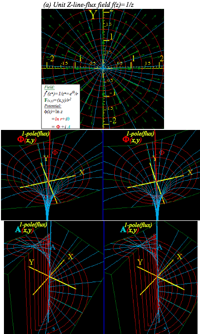
Fig. 10.10(a) Real unit line-source (a=1) with diverging F-field resembling E-field of electric line-charge.
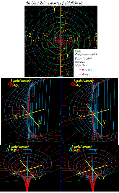
Fig. 10.10(b) Imaginary line-source (a=i) with curling F-field resembling B-field of electric line-current.
Complex derivatives give 2D multipole fields
Of
all integer-power-law field functions f(z)=zn of z,
only a/z
=az-1 has a
non-power-law multi-valued integral and potential ![]() (10.38) and
non-zero flux-work-loop integral
(10.38) and
non-zero flux-work-loop integral ![]() (10.39).
This f(z)=az-1 is a 2D line monopole field and
(10.39).
This f(z)=az-1 is a 2D line monopole field and ![]() is its monopole potential of source strength a.
is its monopole potential of source strength a.
![]() (10.40a)
(10.40a) ![]() (10.40b)
(10.40b)
Now let these two line-sources of equal but opposite source constants +a and –a be located at z=±Ä/2 thus separated by a small interval Ä. This sum (actually difference) of f1-pole-fields is called a dipole field.
![]()
![]()
If interval Ä is tiny and is divided out we get a point-dipole field f2-pole that is the z-derivative of f1-pole.
![]() (10. 41a)
(10. 41a) ![]() (10.
41b)
(10.
41b)
A point-dipole potential ö2-pole (whose z-derivative is f2-pole) is a z-derivative of ö1-pole. Pair (10. 41) looks like a Coulomb force (9.1) and potential (9.2) of 3D point monopoles. However, 2D dipole field (10. 41a) is quite different as is 2D potential (10. 41b) whose Ö=const. and A=const. lines make a circle-net in Fig. 10.11.
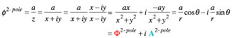 (10.42)
(Note that complex z=x+iy is cleared from the denominator by using z*=x-iy to give real r2= z*z=x2+y2.)
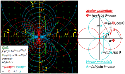
Fig. 10.11 Dipole F-field f(z)=1/z2 and scalar potential (Ö=const.)-circles orthogonal to (A=const.)-circles.
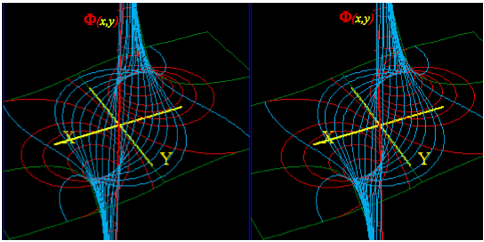
Fig. 10.12 Stereo 3D plot of dipole ö(z)=1/z scalar potential Ö(x,y) with A-streamlines between poles.
Complex power series are 2D multipole expansions
A z-derivative turns 1-pole fields into 2-pole fields in (10. 41). It makes a copy of 1-pole in (10. 40) with a sign change and puts the (-)copy very near the original. What if we put a (-)copy of a 2-pole near its original? Well, the result is 4-pole or quadrupole field f4-pole and potential ö4-pole, each a z-derivative of f2-pole and ö2-pole.
![]() (10.43a)
(10.43a) ![]() (10.43b)
(10.43b)
Fig. 10.13 shows 4-pole structure. Two +∞-poles loom above Y-axis and two -∞-poles lurk below X-axis . The F-field vectors and their A-streamlines are shown running at 90° to Ö-equipotential lines in Fig. 10.13.
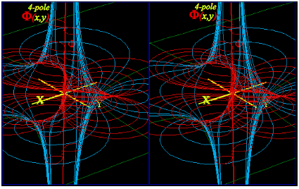
Fig. 10.13 Stereo 3D plot of quadrupole ö(z)=1/z2 scalar potential Ö(x,y) with A-streamlines between poles.
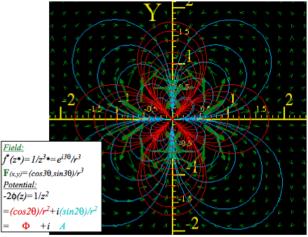
Fig. 10.14 F-field f(z)=1/z3 of 4-pole with scalar (Ö=const.)-equipotentials normal to (A=const.)-streamlines.
A
field
f(z) with sources only at
origin (z=0) or at infinity (z=∞) may be given by power series that
generalize Maclaurin series derived in (10.11) by using both positive and
negative powers z±n. Series Óa±nz±n is called a Laurent series or multipole expansion
(10.44) of a given complex field function f(z) around z=0. All field terms am-1zm-1 except 1-pole ![]() have
potential term am-1zm/m of a 2m-pole at z=0 (z=∞) for m<0 (m>0).
have
potential term am-1zm/m of a 2m-pole at z=0 (z=∞) for m<0 (m>0).
 (10.44)
The
unique 1-pole(20-pole)öterm ![]() is not a constant a-1z0=a-1. (Constantö has no field:
is not a constant a-1z0=a-1. (Constantö has no field:![]() ) Also a 1-pole at
z=∞ gives zero field near
z=0. However, a 21-pole at z=∞ gives a constant field f(z)=a0 near z=0. A quadrupole (22-pole) at z=∞ gives the linear field f(z)=a1z shown if Fig. 10.7, but a 22-pole at z=0 gives the field a-3z-3 in Fig. 10.14. Octupoles (23-poles)
at z=∞ (or z=0) give a2z2 (or a-4z-4), and so on for m=4,5,…
) Also a 1-pole at
z=∞ gives zero field near
z=0. However, a 21-pole at z=∞ gives a constant field f(z)=a0 near z=0. A quadrupole (22-pole) at z=∞ gives the linear field f(z)=a1z shown if Fig. 10.7, but a 22-pole at z=0 gives the field a-3z-3 in Fig. 10.14. Octupoles (23-poles)
at z=∞ (or z=0) give a2z2 (or a-4z-4), and so on for m=4,5,…
Complex 1/z gives stereographic projection
The potential öexpansion is most useful for revealing multi-pole structure. A negative power öterm a-m-1z-m/m belongs to a 2m-pole at z=0. A positive power öterm am-1zm/m belong to a 2m-pole at z=∞. Pole field geometry involves mapping z-points onto a sphere so z=0 is its North Pole and z=∞ is its South Pole in Fig. 10.15. There a stereographic projection maps a point z=x+iy on the z-plane tangent to North Pole into a point w=1/z=u+iv in the inverse w-plane tangent to the South Pole. The map geometry uses an inscribed rectangle. A pair of red unit circles |z|=1 and |w|=1 map into each other. Any point z inside the |z|=1 circle maps into a point w outside the |w|=1 circle as shown and vice-versa outside z maps to inside w.

Fig. 10.15 Stereographic projection of z-plane through a unit-diameter sphere to inverse 1/z=w-plane.
Replacing z with w=z-1 in (10.13) switches positive multi-pole-m terms in potential ö with negative ones.
![]() (from (10.44))
(from (10.44))
![]() (with z=w-1)
(with z=w-1)
![]() (with w=z-1)
(with w=z-1)
But,
the unique monopole source term stays put with only a sign change (![]() ) as seen in
Fig. 10.16a. Constant field f=a0 in (10.44) appears if there is a dipole
at the South Pole and, vice-versa, a dipole field at the North Pole appears to be a constant
field near the South Pole as seen in Fig. 10.16b.
) as seen in
Fig. 10.16a. Constant field f=a0 in (10.44) appears if there is a dipole
at the South Pole and, vice-versa, a dipole field at the North Pole appears to be a constant
field near the South Pole as seen in Fig. 10.16b.
Of all 2m-pole field terms am-1zm-1, only the m=0 monopole a-1z-1 has a non-zero loop integral (10.39).
![]()
![]()
This m=1-pole constant-a-1 formula is just the first in a series of Laurent coefficient expressions.
![]()
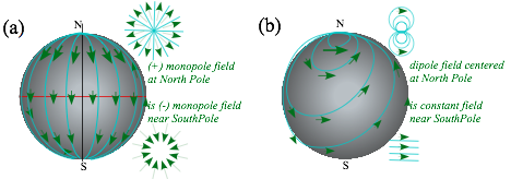
Fig. 10.16 Projective sphere view of North Pole (z=0) sources. (a) monopole (b) dipole.
Source
analysis starts with 1-pole loop integrals ![]() or,
with origin shifted
or,
with origin shifted ![]() .
They hold for any loop around point-a. A continuous function f(z) is just f(a) on a tiny circle around point-a.
.
They hold for any loop around point-a. A continuous function f(z) is just f(a) on a tiny circle around point-a.
![]() (10.45a)
(10.45a)
![]() (10.45b)
(10.45b)
The f(a) result is called a Cauchy integral. Then repeated a-derivatives gives a sequence of them.
![]()
This leads to a general Taylor-Laurent power series expansion of function f(z) around point-a.
![]() (10.45c)
(10.45c)
If the function f(z) has no poles inside the contour then only positive powers n>0 are needed in its expansion and the series above reduces to a Taylor series or (if a=0) a Maclaurin series like (10.12) derived previously. There the nth expansion coefficient an is given by nth derivative of f(z) as in (10.45c) above. Otherwise, negative powers are needed with coefficients given by nth order pole loop integrals above.
This represents just a “tip of an iceberg” for an enormous subject of complex analysis. We shall use only tiny portions of this grand mathematical subject, and later we will consider generalizations of complex numbers to hyper-complex quaternions and spinor operators in Unit 4. This takes the analysis from a 2D framework into a 3D and 4D description that is more like the space-time we seem to live in.
Exercises
Construct dipole function geometry of Fig. 10.11.
Chapter 11. Oscillation, Rotation, and Angular Momentum
We last left the neutron starlet orbiting on an ellipse inside the Earth in Fig. 9.10 according to
x = a cos ù t (9.13a)repeated y = b sin ù t (9.13b) repeated
Here we show a Kepler construction for such an orbit that works for any ellipse. (It is like Fig. 3.6.) We also expose more geometry of velocity-velocity KE-ellipses used to introduce Lagrangian, Hamiltonian, action, and contact transformations in the following Chapter 12. That leads to more efficient ways to treat orbits.
Keplerian construction of elliptic oscillator orbits
To be historically correct, Kepler was concerned with elliptic orbits that lie outside of the Earth not the inside-Earth orbits in a linear force law F(r) = -kr that we plotted. As we will show in Unit. 5, outside orbits in a Coulomb force law F(r) = -kr-2 also have elliptic orbits, albeit with origin r=0 at a focal point. That’s a little more complicated. So, we first study the easier inside-Earth orbit ellipses that have r=0 centered. This gives some properties of their country cousins who live well outside the city limits.
Elementary ellipse construction
Fig. 11.1 shows an easy 4-step construction for points on a (major-radius=a, minor radius=b)-ellipse. Note that you don’t have to draw OA first. Pick a vertical (AX) or a horizontal (BR) line first and then find the others including the OA radius that goes with your choice. Given x or y, you find t or vice versa.
The big a-circle acts like a clock dial. The x-shadow or projection of the clock dial is x = a cosù t and every mass that starts at x=a at zero-x-velocity will forever live in the shadow of the tip of the clock hand. This includes any ellipse with semi-major axis a, but arbitrary semi-minor axis b.
The ellipse in Fig. 11.1 has b=1 and a= 2.2. The speed of the orbiting mass can be estimated by the space between positions at equal time intervals. Speed is smaller as the mass rounds the long end of the ellipse than it is as it zips by the minor axis. In fact we shall show that it is exactly 2.2 times faster, a result that is attributed to Johannes Kepler and is the result of the conservation of angular momentum.
As mentioned before after Fig. 9.8, all orbits have the same period, and the mass that tunnels through the Earth center at the bottom of Fig. 11.1 has exactly the same x-equation x = a cos ù t as the ellipse-following mass above it. They differ only in their y-equation y = b sin ù t ; in the first case the tunneling mass has b=0. A circular orbit would have b=a, but its x-equation would be the same. Note how the radius vector r of the mass lags behind the ù t-clock-hand at first, but then at the b-axis low point (perigee) of the orbit it catches up and passes until the clock hand catches it again at the other a-axis high point (apogee or “up-ogee”). This leap-frog motion relates to one of Kepler’s most famous laws and the conservation of angular momentum as will be reviewed shortly.
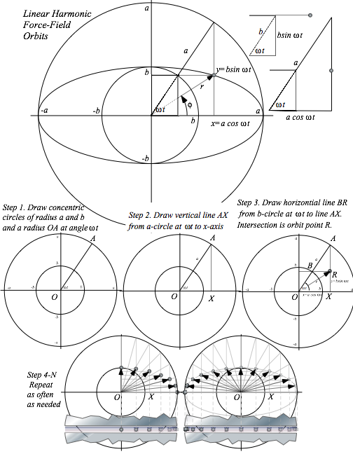
Fig. 11.1. Harmonic force-field elliptical orbit construction.
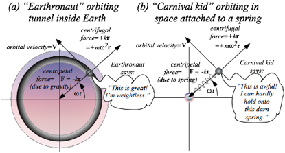
Fig. 11.2 Two different systems with identical oscillator orbits. (a) Inside Earth, (b) Mass on spring.
Orbiting versus rotating: Centripetal versus centrifugal
Imagine an “Earthronaut” orbits inside the Earth in a linear gravity field F=-kr, as sketched in Fig. 11.2(a). (Recall “starlet” in Fig. 9.9.) Let’s compare to a kid rotating in a carnival ride at one end of a spring as the other end pivots frictionlessly about a fixed point. (See Fig. 11.2(b).) Each m does the same orbit, but there’s a big difference. You’d notice it if you were the mass m.
The Earthronaut feels weightless like astronauts in orbit. But the rotating kid feels a great outward pull, a centrifugal or center-fleeing force F=+kr. Stop the rotating “carnival kid” and the centrifugal force goes away. If the kid lets go he feels weightless in space. Stop the orbiting Earthronaut and the inward tug F=-kr by the centripetal or center-pulling force of gravity returns as the Earthronaut resumes weighing mg=kr. Earth gravity is no longer cancelled by inertial reaction force and he cannot let go of g.
An orbiting Earthronaut feels weightless because the two forces, outward centrifugal F=+kr and inward centripetal F=-kr , cancel to zero for body mass m or any part of it. On the other hand, the carnival kid feels stretched out by two equal and opposite forces, again an outward centrifugal F=+kr pulling the kid up opposes an inward centripetal F=-kr provided by the spring that the kid is holding onto.
In each case, outward centrifugal F=kr is due to rotation at angular rate ù around a circle of radius r at velocity V= ù r. The angular rate ù is the Earth or spring oscillator frequency from (9.9) or (10.23).
![]() (11.2a) or:
(11.2a) or:
![]() (11.2b)
(11.2b)
Centrifugal force formulas that result are among the most famous formulas in rotational mechanics.
Fcentrifugal = k r = mù2 r = m V2/r where: V= ù r (11.3a)
Removing the mass m gives the also-famous centrifugal acceleration formulas.
acentrifugal = ù2 r = V2/r where: V= ù r (11.3b)
A geometer likes to imagine fitting a curve by circles at each point with smaller circles fitting more curvy points. These so-called circles of curvature become bigger circles as a curve straightens out. A geometer-physicist does the same, but imagines driving at a constant speed V along the curve with an accelerometer to measure transverse centrifugal acceleration acentrifugal. By (11.3b) the accelerometer reads V2/rcurv outward from a curve if the car is rounding a circle of radius rcurv = V2/ acentrifugal with its center that distance inside the curve. The acentrifugal-reading is inversely proportional to radius of curvature for fixed linear velocity V, but directly proportional to it for fixed angular velocity ù.
rcurv = V2/acentrifugal= acentrifugal /ù2 where: V= ù rcurv (11.3c)
It is a strange but useful view of a curve! The physicist imagines riding a carnival Merry-Go-Round whose rim speed V is constant but whose radius and center keep changing! If the road straightens to veer the other way, the Merry-Go-Round center becomes infinite and reappears on the other side.
Note that road speed V is constant in the physicist’s image. There’s no acceleration along the road, only perpendicular to it. However, in real orbits around planets or springs, velocity V holds constant only for circular orbits or, ever so briefly, at special points on elliptical ones. One special point is a low point or perigee. Another is a high point or apogee. (Think “ap” means “up” in space lingo.)
An astronaut in an elliptic orbit or a mass on an elliptic oscillator orbit like Fig. 11.1 will increase speed (accelerate) as it “falls” from the high-point apogee on the x-axis toward the low-point perigee on the y-axis. Then it will decrease speed (decelerate) as it rises back to apogee. Only at apogee or perigee is the speed momentarily constant. Then, and only then, is force and acceleration perpendicular to the flight path. In between, the F=-kr vector makes an angle è with velocity V that is not 90° so the work (dW= F•dr= |Fdr| cosè) or power (P= F•V= |FV| cosè) is non-zero so kinetic energy varies.
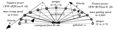
Fig. 11.3 Elliptic orbit force, velocity, and power variation.
More inertial forces: Coriolis and tidal forces
Carnival kid would feel even more forces on an elliptic orbit, though the Earthronaut may still be nearly weightless. Gravitational force is balanced by centrifugal force and, between apogee and perigee, by another kind of inertial force called the Coriolis force that opposes orbital velocity.
To visualize Coriolis force imagine what you would feel walking along a radial railing toward the center of a Merry-Go-Round rotating to your right as in Fig. 11.4(a). The railing pushes you left (against the rotation) to slow you down to zero speed when or if you get to the center of the Merry-Go-Round. The Coriolis force is proportional to your radial walking speed. Stop walking inward and all you feel is the usual centrifugal force pulling back out along the radial railing path. Walk back out and Coriolis pushes you to the right to get you up to the Merry-Go-Round rotation speed at each point.
Coriolis forces can make you dizzy and nauseous. Centrifugal force is steady as long as you are fixed to the Merry-Go-Round. But, if you just turn your head, the fluids in your inner ear get a kick perpendicular to the direction of motion and they’re not used to that.
Fig. 11.4(b) shows centrifugal and Coriolis forces of an inward falling orbiting mass analogous to that of the Merry-Go-Round. The Coriolis force acts oppositely to orbital velocity V on the way in and then acts with V on the way out in Fig. 11.4(c). At apogee or perigee in Fig. 11.4(d) there is centrifugal-centripetal force but no Coriolis force since the mass momentarily stops its radial motion.
The Earthronaut may not feel centrifugal or Coriolis forces if every atom almost perfectly balances inertial force by equal and opposite gravitational force to make a feel-force-free orbit. But, “almost” is not zero! Suppose our astronaut is on a 1 kHz neutron star orbit. (That’s ù=2000π.) He (or she) is toast and jelly due to what is called tidal force. Only the astronaut’s center-of-gravity is right on a feel-force-free elliptic orbit. For the rest that’s the wrong ellipse! The poor astronaut’s left and right hands (and ears and other bilateral pieces of anatomy) try to change places 2000 times per second as disparate free-fall orbits crisscross back-and-forth twice each period. Really barf!
The k-constant or spring constant for an oscillator tidal force felt by a neutron-astronaut (who will be reduced to a “neuternaut” by one orbit) is given by (11.2b).
k=mù 2= m6.282 E6 (N/m) for: ù=2000π
That is almost 40 million Newtons (10 million lbs. or 5 thousand tons) for each kilogram of mass a meter off-center or 50 tons of pressure just on a 1 cm-sized fingertip.
Quite a number of astrophysical effects are due to tidal forces like ocean tides. The Moon presents one face because its tides due to Earth have wasted as much of its rotational energy as possible. So it’s locked relative to Earth with only slight (but interesting) nutational wobbling due partly to its eccentric orbit.
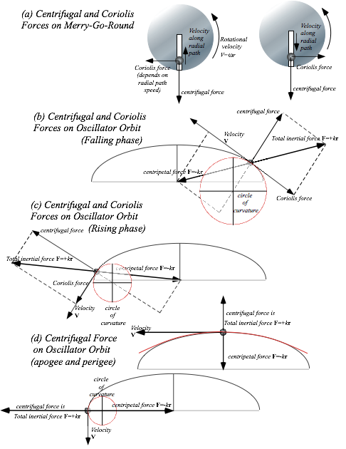
Fig. 11.4 Centrifugal and Coriolis forces. (a) Simple Merry-Go-Round. (b-d) Various orbital phases.
Vector analysis and geometry of elliptic oscillator orbit
An ellipse orbit is characterized using vectors r, v, and F= ma that are arrows in Fig. 11.4. First, there is the location, position, or radius vector r that we found in (9.13).
![]() (11.5a)
(11.5a)
Second,
there is the rate, speed, or velocity vector
v that is a 1st time derivative![]() .
.
![]() (11.5b)
(11.5b)
Unit-m force F is proportional to 2nd derivative (Change-of-velocity is acceleration a) and is just -ù2r.
![]() (11.5b)
(11.5b)
Then the 3rd derivative (Change-of-acceleration is jerk j), is just -ù2v,
![]() (11.5c)
(11.5c)
and finally the 4th derivative (Change-of-jerk is inauguration i), equals the r-vector with a scale factor ù4.
![]() (11.5d)Linear
Hooke force F=-kr gives F=ma=-kr
then a=-ù2r
then j= -ù2v,
and so on. The 5th derivative (Change-of-inauguration is revolution) is just ù5v. As plotted in Fig. 11.5, the four
vectors r, v/ù, a/ù2, and j/ù3 follow each other on one
ellipse orbit of Fig. 11.1 taking turns to slow down then to speed up.
(11.5d)Linear
Hooke force F=-kr gives F=ma=-kr
then a=-ù2r
then j= -ù2v,
and so on. The 5th derivative (Change-of-inauguration is revolution) is just ù5v. As plotted in Fig. 11.5, the four
vectors r, v/ù, a/ù2, and j/ù3 follow each other on one
ellipse orbit of Fig. 11.1 taking turns to slow down then to speed up.
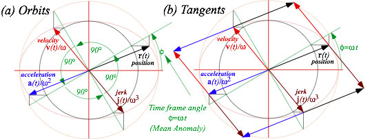
Fig. 11.5 Harmonic oscillator orbit ellipse (a) All derivatives follow same orbit. (b) Related tangents.
Each of the four vectors r, v/ù, a/ù2, and j/ù3 in Fig. 11.5 has a time-phase angle or mean anomaly value ö=ùt that is spaced at π/2 intervals ùt, ùt+ð/2, ùt+ð, and ùt+3ð/2, respectively, as listed below.
 (11.6a)
 (11.6b)
 (11.6c)
 (11.6d)
Matrix operations and dual quadratic forms
Ellipse
equation ![]() may
be written using a matrix
may
be written using a matrix ![]() on
position vector
on
position vector ![]() .
.
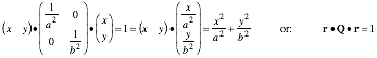 (11.7)
Function r•Q•r is a quadratic
form QF. QF’s are useful to mechanics and their powerful
geometry will be demonstrated for orbit ellipses and later for KE ellipses.
First note that if a matrix ![]() acts
on a radial position vector
acts
on a radial position vector ![]() it
gives a vector p perpendicular to ellipse tangent
it
gives a vector p perpendicular to ellipse tangent ![]()
![]() at r.
at r.
![]() (11.8a)
(11.8a)
p is
perpendicular, that is, orthogonal to the velocity vector v=![]() (11.5b) as
seen here and in Fig. 11.6.
(11.5b) as
seen here and in Fig. 11.6.
![]() (11.8b)
(11.8b)
These p-vectors define their own ellipse r•Q-1•r=1 of an inverse quadratic formQ-1F. Its radii are inverse (1/a,1/b) of the original Q-ellipse radii(a,b) in (11.7). The Q-1F-ellipse is the dashed oval in Fig. 11.6.
![]() (11.9)
(11.9)
Inverse operation Q-1•p on perpendicular p returns the radial position vector r on the Q-ellipse.
![]() (11.10a)
(11.10a)
r is orthogonal to the
Q-1F-ellipse tangent![]() , just as p
is orthogonal to the QF-ellipse tangent
, just as p
is orthogonal to the QF-ellipse tangent![]() in (11.8b).
in (11.8b).
![]() (11.10b)
(11.10b)
Vectors p and r
maintain a unit mutual projection, that is, dot-products p•r
and![]() always
equal 1.
always
equal 1.
![]() (11.10c)
(11.10c)
Fig. 11.6b shows a geometric-algebraic symmetry where ellipse plots are scaled by geometric mean S=√(ab) so that each scaled major radius aS=a/S is the inverse of its minor radius bS=b/S and aS bS=1.
aS=a/S=√(a/b)=1/bS (11.11a) bS=b/S=√(b/a) =1/aS (11.11b)
Then inverse ellipse r•Q-1•r=1 is an axis switch (![]() ) or 90°
rotation of ellipse r•Q•r=1 by
symmetry.
) or 90°
rotation of ellipse r•Q•r=1 by
symmetry.
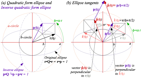
Fig. 11.6 Ellipse vectors and tangents for quadratic forms. (a) Ellipse vectors. (b) Tangent geometry.
Slope multiplication and eigenvectors
Matrix![]() or
or ![]() acting
on a vector
acting
on a vector ![]() multiplies
its slope
multiplies
its slope![]() by a/b or b/a respectively.
by a/b or b/a respectively.
![]() (11.12a)
(11.12a) ![]() (11.12b)
(11.12b)
Matrix![]() or
or ![]() multiplies
slope by a2/b2 as in (11.8a) or b2/a2
as in (11.10a).
multiplies
slope by a2/b2 as in (11.8a) or b2/a2
as in (11.10a).
![]() (11.13a)
(11.13a) ![]()
![]() (11.13b)
(11.13b)
Only
vectors of slope zero or infinity, such as ![]() or
or ![]() , are immune
to slope-change by R or R-1.
, are immune
to slope-change by R or R-1.
![]() (11.14a)
(11.14a) ![]() (11.14b)
(11.14b)
They are
called eigenvectors of R-1 or any power ![]() of R or R-1.
of R or R-1.
![]() (11.15a)
(11.15a) ![]() (11.15b)
(11.15b)
![]() (11.15c)
(11.15c) ![]() (11.15d)
(11.15d)
These
special vectors are operator Rp’s
own base vectors for any power p. Eigenvector is German for “own-vector.”
Base vectors ![]() and
and![]() define a
Qp-and-Rp-ellipse’s own major
and minor axial directions. The axial radii a
and b are the eigenvalues of
R-1 in (11.14). Powers
ap and bp
are eigenvalues of R-p.
define a
Qp-and-Rp-ellipse’s own major
and minor axial directions. The axial radii a
and b are the eigenvalues of
R-1 in (11.14). Powers
ap and bp
are eigenvalues of R-p.
Each action
of R (or Q) on vector r grows its slope by a/b (or a2/b2)
so it approaches eigenvector![]() while R-1 and Q-1 make it approach eigenvector
while R-1 and Q-1 make it approach eigenvector
![]() . Each slope
polar angle ök
plotted in Fig. 11.7 is obtained from its neighbors ök-1 and ök+1
by inscribing a rectangle between r=a and r=b with its main
diagonal on the ök
line. Lower and upper corners on the cross-diagonal give radial position r(ök-1) on the Q-ellipse and
perpendicular p(ök+1)
on the Q-1-ellipse, respectively, following Fig. 11.1 and (11.13).
. Each slope
polar angle ök
plotted in Fig. 11.7 is obtained from its neighbors ök-1 and ök+1
by inscribing a rectangle between r=a and r=b with its main
diagonal on the ök
line. Lower and upper corners on the cross-diagonal give radial position r(ök-1) on the Q-ellipse and
perpendicular p(ök+1)
on the Q-1-ellipse, respectively, following Fig. 11.1 and (11.13).
p(ök+1)=Q•r(ök-1) where: tan(ök+1)= (a/b) 2 tan(ök-1) (11.16)
For the kth
triad, angle ök =ùtk is the “timer” angle
and polar angle of main diagonal while ök-1
is the polar angle of radial position r(ök-1)
and ök+1 is the polar
angle of perpendicular p(ök+1)
to velocity ![]() (ök-1)= v(tk).
(ök-1)= v(tk).
p(ök+1)•![]() (ök-1)=0=
(ök-1)=0= ![]() (ök+1)•
(ök+1)•![]() (ök-1) (11.17a) p(ök+1)•r(ök-1)=1 (11.17b)
(ök-1) (11.17a) p(ök+1)•r(ök-1)=1 (11.17b)
This restates the duality relations (11.10) for an entire sequence, part of which is shown by Fig. 11.7b.
A
{ök} sequence may
start on any angle but a choice ö0=ð/4 in Fig. 11.7 gives symmetric
results. Also, we may let: ab=1 and: ![]() below by
assuming unit scale S=1 in (11.11).
below by
assuming unit scale S=1 in (11.11).
![]()
![]()
![]()
![]() (11.18a)
(11.18a) ![]() (11.18b)
(11.18b) ![]() (11.18c)
(11.18c)
![]()
![]()
![]()
Triads {rk+1,rk,rk-1} and {pk+1,pk,pk-1} of vectors rk=r(ök) and pk=p(ök) are given for ö0=ð/4.
![]()
![]()
![]() (11.19)
(11.19)
Each triad
{rk+1,rk,rk-1}
easily gives the tangent vk-1=v(ök-1)=![]() that
contacts the Q-ellipse at rk-1. An arc
by rk intersects rk+1
where vk-1 is perpendicular to rk+1
or pk+1=p(ök+1).
(See Fig. 11.7a and exercises.)
that
contacts the Q-ellipse at rk-1. An arc
by rk intersects rk+1
where vk-1 is perpendicular to rk+1
or pk+1=p(ök+1).
(See Fig. 11.7a and exercises.)
So far the ellipse axes line up with the Cartesian coordinate axes of a standard page. Ellipses in other bases may be rotated, and certainly an orbit of an isotropic oscillator may choose any direction for its axes. The following general 2D quadratic form gives a rotated conic section (ellipse or hyperbola).
![]() (11.20)
(11.20)
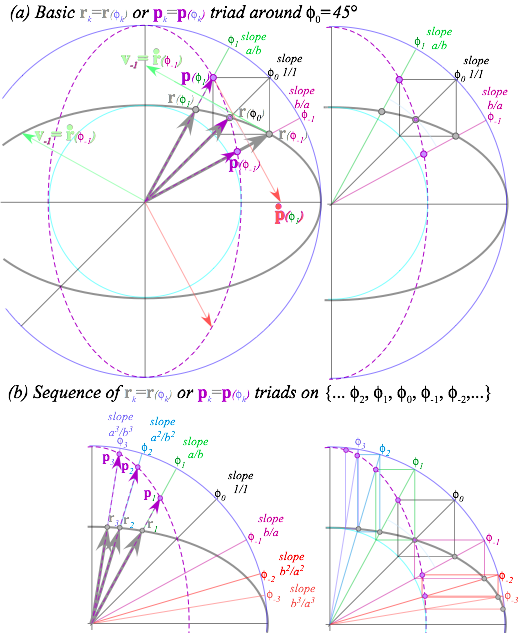
Fig. 11.7 Triad sequence geometry of radial position vector r(ön-1) and tangent-perpendicular p(ön+1).
However, all the relative geometric properties such as their tangent geometry are the same in all bases. It’s abstract vector equation 1=r•Q•r looks the same in any coordinate base system, but the matrix components may include non-zero off-diagonal elements B≠0 that indicate it is a rotated ellipse.
Angular momentum and Kepler’s law
The shape and rotational orientation of an isotropic oscillator orbit ellipse is constant with time. The cross product of rxv of position and velocity is also a constant of the motion by (11.5). (See App. 1.A.)
![]() (11.21)
(11.21)
The quantity L=m rxv is called orbital angular momentum. It’s conserved as mass m orbits.
![]() (11.22)
(11.22)
It means the area of r+v or r-v triangles, as discussed in Appendix 1.A, are constant on an orbit as indicated in Fig. 11.8 below. Area enclosed by r and v is proportional to the area π ab of the whole orbit.
![]()
Fig. 11.8 Vector r+v and r-v parallelogram and triangle areas are constant all during orbit.
By (11.22), velocity at perigee (x=0,y=b) is vb=L/mb=aù. At apogee it slows to va=L/ma=bù. This is consistent with velocity formula (11.5b). Constant momentum relates to Kepler’s Law: the radius r-vector sweeps the same area every second or every hour and equal time means equal area.
This is true since the triangle made of r and dr=v dt has the same area 1/2rxv dt = (L/m)dt for the same time interval dt. This law applies to any central force that is a function of radius r alone, not just the oscillator force F=-k·r. This includes the Coulomb force F=-k/r2, which is the only other force to have elliptical orbits that maintain their orientation.
The oscillator and Coulomb forces each have hidden symmetry beyond their Keplerian rotational isotropy that conserves angular momentum and this makes their orbits have simple geometric properties. This extra symmetry will be analyzed in units 4 and 5.
Flight of a stick: Introducing geometry of cycloids
If linear momentum and
angular momentum are conserved they often do so together. As an example, we
consider the flight of a rigid rod or stick in free space. Flying rods are
treated in Sec. 6.4 of the rigid body unit (Unit 6) but elementary aspects of
rigid body motion are easy to derive and they display cycloid geometry that is
useful for several classical mechanical phenomena. A mass m rotating on
a circle of radius r with angular velocity ù has a linear tangential velocity V=ù·r and
kinetic energy ![]() .
(Recall (9.10) for orbiting starlet.) An angular form is derived here again.
.
(Recall (9.10) for orbiting starlet.) An angular form is derived here again.
![]() (11.23)
(11.23)
Circular orbiter angular momentum (from (11.22) above) takes an angular form, too.
![]() (11.24)
(11.24)
In each the
point mass rotational inertia ![]() replaces
linear mass m while angular
velocity ù replaces V.
replaces
linear mass m while angular
velocity ù replaces V.
A
rod or lever of length l
rotating about one end is viewed as an integral from r=0 to r=l of its mass points ![]() each of
infinitesimal inertia
each of
infinitesimal inertia ![]() .
Density ñ is the rod’s
total mass M per length l, and that is assumed
to be uniform. Total inertia follows from taking the integral over its length.
.
Density ñ is the rod’s
total mass M per length l, and that is assumed
to be uniform. Total inertia follows from taking the integral over its length.
![]() (11.25)
(11.25)
This
inertial formula is true for two identical rods of length l welded end-to-end and
rotating about that point. Now mass M
is that of the total system. In free space the straight welded rod will rotate
naturally with constant angular velocity ù about the welded point at its center of mass and
that center travels at a constant velocity ![]() until
hit by an outside force.
until
hit by an outside force.
Then free-space paths of each point on the rod, including its center-of-mass, are generalized cycloids such as are shown in Fig. 11.9. There are two dots on the rod (a red dot • and a green dot •) that follow normal cycloids. Each comes to a complete stop at a cycloid cusp (as green dot • is in the lower center of the figure) while the opposite dot is just reaching its maximum velocity (as red dot • is in the upper center of the figure). On left and (later) right sides of Fig. 11.9 is similar with rod flipped.
Imagine dot • and dot • are pieces of gum stuck to opposite sides of a tire (green circle of radius p in Fig. 11.9) rolling left-to-right along a line (“road”) with rod CM point attached at tire center. A blue dot • on one end of the rod is initially above the green dot • (upper left of Fig. 11.9) while the rod’s lower end has a violet dot • attached below the red dot • where the tire initially meets the road. Rod points outside tire radius (blue dot • and violet dot •) trace curlate cycloids. Inside points (CM and yellow dot •) trace prolate cycloids. The CM just follows a straight line at constant speed. Tire radius p depends on hit-height h above CM point where momentum impulse Ð is delivered in Fig. 11.10. However, regardless of h, the CM point will travel at constant linear velocity V=Ð/M while the rod conserves linear momentum Ð=MV.
Center of percussion, radius of gyration, and “sweet-spot”
Angular
velocity ù relates to
hit-height h factor in angular
momentum Iù=Ë=Ðh
and to tire radius p where red dot
• on tire comes to rest on road, and velocity ù·p=Ðh·p/I
due to rotation cancels velocity V=Ð/M due to translation. This gives relation h·p=I/M.
Rod inertia ![]() then
gives relation
then
gives relation ![]() between
hit-height h and radius p of percussion
for rod of radius l. We call hit
point h a “sweet-spot” for point P and vice-versa.
between
hit-height h and radius p of percussion
for rod of radius l. We call hit
point h a “sweet-spot” for point P and vice-versa.
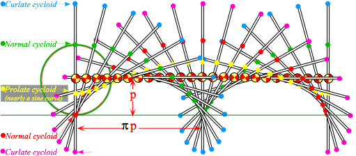
Fig. 11.9 Free flying rod of length L=2l “rolls” left-to-right on “tire” of radius p.
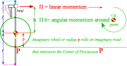
Fig. 11.10 Impulse hit-height h relates to rod radius l and percussion radius p of rolling “tire.”
If the hit-height h is zero then percussion radius p is infinite and all points of the rod follow straight parallel paths since there will then be zero rod rotational velocity ù and zero angular momentum Ë=Ðh. Only linear velocity V=Ð/M would be nonzero then. If the hit-height h is equal to l (the maximum practical value of h is the radius l of rod) then the percussion radius is p=l/3, its minimum practical value.
Reducing h increases p proportionally. The two are equal at the value p=l/√3=h=0.866l which is called the radius of gyration of the rod. Reducing hit-height h further to l/2 and l/3 increases the percussion radius p to p=2l/3 and p=l, respectively. The percussion point is where you can hold the lever and feel the very least recoil during the hit. In fact, the dynamics at a normal cycloid cusp point at radius p in Fig. 11.9 amounts to a gentle tug along the lever but no force perpendicular to it.
Baseball bats are made thicker at the hitting end to accommodate h and p points further from the ends than allowed by p=h=0.866l. Cricket bats, on the other hand, seem to be more like sticks.
Exercise 1.11.1
Quadratic
form matrices are generally non-diagonal ![]() . If Q has positive
eigenvalues 1/a2 and 1/b2 its form is called positive definite and r•Q•r =1 gives an ellipse
rotated by angle è with radii a and b. So does r•Q-1•r =1.
. If Q has positive
eigenvalues 1/a2 and 1/b2 its form is called positive definite and r•Q•r =1 gives an ellipse
rotated by angle è with radii a and b. So does r•Q-1•r =1.
(a)
Derive relations between matrix parameters {A,B,D} and ellipse parameters {a,b, è }. (Hint: Start with diagonal matrix and
rotate it to Q´=R·Q·R-1 by applying rotation
transformation matrices ![]() and
and
![]() .)
.)
(b)
Show TraceQ and detQ (or TraceQ-1 and detQ-1) are invariant to è and relate them to conserved quantities
such as total energy ![]() and orbital
momentum
and orbital
momentum ![]() of isotropic 2D
harmonic oscillator orbit elliptic orbit r(t) in (11.5). Could the energy or momentum of an
isotropic 2D HO orbit depend on orientation angle è ? How or why not?
of isotropic 2D
harmonic oscillator orbit elliptic orbit r(t) in (11.5). Could the energy or momentum of an
isotropic 2D HO orbit depend on orientation angle è ? How or why not?
(c) Suppose Q’s eigenvalues were 1/a2 and -1/b2. What curve is r•Q•r =1? Plot for a=1=b and è = 45°.
Exercise1.11.2
Recall
Fig. 11.7 geometric sequence {r-3, r-2, r-1, r0, r1, r2, r3,…} of ellipse radii rk=r(ök) and
perpendicular-to-tangents
pk+2 =Q•rk defined by quadratic
forms
rk•Q•rk =1= pk•Q-1•pk by ![]() . (Ellipse
radii had ab=1 and 0th
sequence slope was tanö0=1 (ö0=ð/4) but other values work
as well.)
. (Ellipse
radii had ab=1 and 0th
sequence slope was tanö0=1 (ö0=ð/4) but other values work
as well.)
(a)
Construct super-imposed r-ellipse and p-ellipse with at least
seven vectors each for a/b=2 (done in class) and a/b=5/4. Give the vectors rk you draw algebraically
(in terms of a and b) for ![]() and
check k=2 cases numerically with
geometry.
and
check k=2 cases numerically with
geometry.
(b)
Verify duality relations: ![]() and
and
![]() . (For time
derivatives let ù=1.)
. (For time
derivatives let ù=1.)
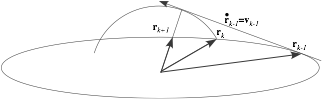
(c)
The text noted that a ellipse tangent vk-1=v(ök-1)=![]() at rk-1 is also tangent to a
circular arc Ck
to k+1
swept by
radius |rk| from the tip of rk to where Ck to k+1 is perpendicular the rk+1-line. Show this implies
a relation
at rk-1 is also tangent to a
circular arc Ck
to k+1
swept by
radius |rk| from the tip of rk to where Ck to k+1 is perpendicular the rk+1-line. Show this implies
a relation
![]() . (Notation
. (Notation
![]() denotes
unit vector:
denotes
unit vector: ![]() )
)
Verify this algebraically and geometrically for the case k=-1 and k=0 using vectors you have derived. Use the result to construct tangents vk contacting each radius {r-3, r-2, r-1, r0, r1, r2, r3,…} on r-ellipse. Place the tangent vectors in r-ellipse.
Chapter 12. Velocity vs momentum functions: Lagrange vs Hamilton
Relating energy ellipses in velocity and momentum space
The ellipse in Fig. 5.1 is skinny and difficult to see. To better view multiple collisions, the v1-v2 axes are rescaled into “quasi-velocities” Vk=vk √mk so the ellipse forms into a nice circle in Fig. 5.2.
![]() where:
where:
![]() and:
and: ![]() (12.1)
(12.1)
The half-power mass scale is helpful. A full power mk-scale converts velocity vk to momentum pk.
![]() where:
where:
![]() and:
and: ![]() (12.2)
(12.2)
Geometry of a p-ellipse is just a flip of the v-ellipse, but there are compelling algebraic reasons for dealing with such alternative functions. In fact two of these functions have famous names attached.
Lagrangian, Estrangian, and Hamiltonian functions
An energy that is an explicit function of velocities is called a Lagrangian function L=L(vk..).
![]() (12.3)
(12.3)
An energy that is an explicit function of momenta is called a Hamiltonian function H=H(pk..).
![]() (12.4)
(12.4)
A compromising function like (12.1) has no famous name so we’ll call it an Estrangian E=E(Vk..).
![]() (12.5)
(12.5)
While all these functions may have the same numerical value for a given situation, the have quite different functional dependence. To emphasize this let us write our first equations of (non)-motion.
![]() (12.6a)
(12.6a) ![]() (12.6b)
(12.6b) ![]() (12.6a)
(12.6a)
The first
two for L and H say that L has no explicit p-dependence
and H has no explicit v-dependence. L may
still vary if p varies but L is not defined by p
and the same for H and v. Calculus distinguishes total derivatives
![]() or
or ![]() from partial
derivatives
from partial
derivatives ![]() or
or![]() and begins
by defining differential chain rule
sums.
and begins
by defining differential chain rule
sums.
![]() (12.7a)
(12.7a) ![]() (12.7a)
(12.7a)
Then L (or H) varies with any variable z such as vk, pk, or time t according to derivative chain rule sums.
![]() (12.7a)
(12.7a) ![]() (12.7a)
(12.7a)
(Imagine L(v...) is “married” to v and H (p...) to p. Dots denote coordinates and time discussed later.)
Neither may use another’s dependents without legal difficulty! Geometry helps clarify this below.
A Lagrangian ellipse plot const. = L(v) in Fig. 12.1a is similar to the superball collision diagram in Fig. 5.1. It is to be compared with the corresponding Estrangian ellipse (circle) plot const. = E(V) in Fig. 12.1b and the Hamiltonian ellipse plot const. = H(p) in Fig. 12.1c. COM and collision line slopes are compared.
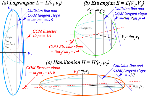
Fig. 12.1 KE ellipse functions related by scale. (a) L in velocity vk space. (b) E in Vk. (c) H in pk.
Functions L, E, and H are quadratic forms of vectors v, V=R•v, and p=M•v=R2•v, respectively.
![]() (12.8a)
(12.8a) ![]() (12.8b)
(12.8b) ![]() (12.8c)
(12.8c)
The
corresponding scaling matrices are powers of the root-mass matrix: R=![]()
![]()
![]()
![]() (12.9)
(12.9)
The 2nd power rescaling M=R2 mass matrix maps L(v) space (a) into Hamiltonian H(p) space (c).
The
p-to-v tangent-normal mapping is analogous to r-to-p
mapping in Fig. 11.6 as displayed in a Fig. 12.2c that overlaps parts (a) and
(c) of Fig. 12.1. Velocity v is a p-space gradient operation ![]() H=
v and thus normal to H-ellipse, and vice-versa for the normal p=
H=
v and thus normal to H-ellipse, and vice-versa for the normal p=![]() L
to the L-ellipse. Matrix notation is given, too.
L
to the L-ellipse. Matrix notation is given, too.
![]() (12.10a)
(12.10a) ![]() (12.10b)
(12.10b)
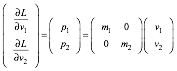 (12.10c)
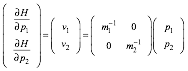 (12.10d)

Fig. 12.2 Tangent-normal mapping between (a) Lagrangian L(v) space and (b) H(p) space.
If mass increases s-times then L-ellipse radii become s times H-ellipse radii. (d) s=1/2, (e) s=2.
Fig. 12.2 is a top view of L(v)-vs-v and H(p)-vs-p plots. Side views are shown and discussed below.
Legendre contact transformations
Given mapping ![]() or
inverse
or
inverse ![]() ,
it might appear that either quadratic form
,
it might appear that either quadratic form![]() or
or ![]() may be
written simply as
may be
written simply as ![]() or
or
![]() . This
is correct numerically but its calculus is not. Instead, it is
. This
is correct numerically but its calculus is not. Instead, it is ![]() or
else
or
else ![]() that
gives correct derivatives. This results in the Legendre contact transformation between H(p)
and L(v) expressed by the following identical equations.
that
gives correct derivatives. This results in the Legendre contact transformation between H(p)
and L(v) expressed by the following identical equations.
![]() (12.11a)
(12.11a) ![]() (12.11b)
(12.11b)
They give correct
partial derivatives with zero for ![]() and
and ![]() according
to definitions in (12.6), as follows.
according
to definitions in (12.6), as follows.
 (12.12a)
  (12.12b)
The results are the first Hamilton equation and the first Lagrange definition (Recall (12.10). Reversing p and v derivatives gives them again in reverse order but quite consistently.
![]() (12.12c)
(12.12c) ![]() (12.12d)
(12.12d)
Side-view sketches of eqs. (12.11) and (12.12) are given in Fig. 12.3a-b and Fig. 12.4a-b below.
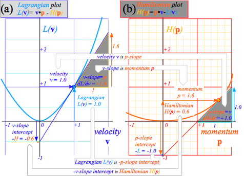
Fig 12.3 Geometry of Legendre contact transformation relating (a) L(v)-vs-v and (b) H(p)-vs-p plots.
Extreme geometry of contact transformations
Contact transformations are among the most enduring and fundamental ideas in either classical or modern physics. Yet few texts on these subjects explain them adequately, if at all. Most can’t even tell why “contact” appears in their name. Our explanation revolves around explicit-function issues involving equations (2.12):
“L(v...) is not function of p, H(p...) is not function of v, yet L(v...), H(p...), p, and v are all related!”
There is method in this madness! One should learn how these ideas “contact” so much of physics.
The
term “contact” refers to a line or curve touching or being tangent-to
another curve. It is opposite to more common cases of crossing or being secant-to
another curve (swordlike). Examples in Fig. 12.4 are based on Fig. 12.3.
Lagrangian side (a) shows secant lines ![]() all of
slope
all of
slope ![]() but
decreasing intercept
but
decreasing intercept ![]() tied
to increasing velocity points
tied
to increasing velocity points![]() leading to a unique tangent to the
leading to a unique tangent to the ![]() curve at tangent contact point
curve at tangent contact point ![]() that
has a max-value
that
has a max-value ![]() of
of
![]() . At that
point the Hamiltonian
. At that
point the Hamiltonian ![]() has
no 1st order variation with respect to velocity, that is,
has
no 1st order variation with respect to velocity, that is, ![]() has zero
1st v-derivative.
has zero
1st v-derivative.
![]() (12.13a)
(12.13a)
Thus ![]() loses its
explicit v-dependence at each tangent
point but
loses its
explicit v-dependence at each tangent
point but![]() does depend on its slope
does depend on its slope![]() .
So also does
.
So also does ![]() lose
its explicit
lose
its explicit ![]() -dependence
at each tangent point but
-dependence
at each tangent point but![]() does depend on that tangent slope
does depend on that tangent slope ![]() .
.
![]() (12.13b)
(12.13b)

Fig 12.4
Geometry of explicit dependence. (a) ![]() loses
loses ![]() dependence.
(b)
dependence.
(b)![]() loses
loses ![]() dependence.
dependence.
Let’s examine more general examples of contact mapping that help clarify its beautiful structure and utility.
General contact transformation geometry
Consider now a contact transformation that relates to some classical physics or to some modern physics while reviewing some sophomore physics. It involves the geometry of volcanic plumes on Io or atomic clouds rising and falling in Earth gravity as sketched in Fig. 12.5a or b, respectively. Each is modeled by a parabolic trajectory fountain in Fig. 12.5c that you may have studied in sophomore physics.
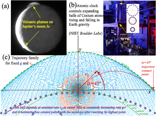
Fig. 12.5 Modeling (a) Io volcano and (b) Atomic clock by (c) trajectories of initial velocity v0 and angle á.
Initial
position x(0)=0=y(0) and velocity ![]() below lead
to a fixed-g trajectory x(t) = (x(t), y(t)).
below lead
to a fixed-g trajectory x(t) = (x(t), y(t)).
![]() (12.14a)
(12.14a) ![]() (12.14b)
(12.14b)
![]()
![]() .
.
The x(t)-solution has time t=x/(v0 cos á) to put in y(t) and get each trajectory y(x) plotted in Fig. 12.5c.
![]() . (12.14c)
. (12.14c)
Each trajectory is a zero value of a Contact Generating Solution S(v0, á : x, y)given by
![]() . (12.15)
. (12.15)
S(v0, á : x, y) maps initial value point (v0=1, á=45°) in Fig. 12.6 onto red trajectory curve y(x) in Fig. 12.5c. A horizontal line of points (same v0 but á varies) fills a region of y(x) space with the v0-trajectory family.
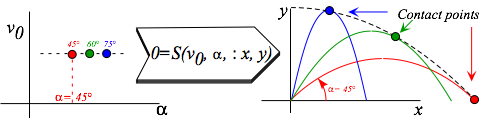
Fig. 12.6 Contact transformation maps point (v0, á) to trajectory of initial velocity v0 and angle á.
Envelopes of the v0-trajectory region contain extremal contact points with each trajectory. Varying á at such a point does not change S so 1st á-derivative of S is zero, quite analogous to zero derivatives in (12.13).
![]() (12.16a)
(12.16a)
![]() (12.16b)
(12.16b)
Solving this equation relates the x-value and the á-value of each contact point for a given fixed v0.
![]() (12.16c)
(12.16c)
If you put this relation into generating function (12.15), it gives the contact envelope function yenv(x).
![]() . (12.17)
. (12.17)
It is the dashed parabolic curve in Fig. 12.5-6 contacting each and (almost) every parabolic trajectory from above. The envelope happens to share the shape of the (á=0)-trajectory hilited in green in Fig. 12.5. That is the single trajectory that never contacts the envelope. Do exercises to see more of this lovely geometry!
A generic general contact transformation S(x,y:X,Y) shown in Fig. 12.7 maps points (xk, yk) in (x, y)-space into points (Xk, Yk) in (X, Y)-space so function y(x) is contact-transformed to function Y(X) there. Such a transformation can occur from one curved set of points to another in the same space as in Huygen’s wavelet view of wave propagation: each wavefront curve at one instant is a contact transform of a wavefront at another time. (Presumably, it’s an earlier time but quantum waves are time reversible.) Contact transform geometry plays such a big role in connecting (contacting) classical and modern physics as we’ll see.
Contact
transforms are key to classical thermodynamics. For example, internal energy U(S,V) is defined as a function of entropy S and volume V. A new function enthalpy H(S,P) depends on entropy and pressure P. It is a Legendre transform H(S,P)=P·V+U of energy U(S,V)
to new variable ![]() .
Except for ±signs, it’s our Hamiltonian H(p)=p·v-L(v) from Lagrangian L(v) to new variable momentum
.
Except for ±signs, it’s our Hamiltonian H(p)=p·v-L(v) from Lagrangian L(v) to new variable momentum![]() .
.

Fig. 12.7 General contact transformation S(x,y:X,Y) maps each point (xk, yk) to a contact point (Xk,Yk).
Let us return briefly to the Legendre-Lagrangian-Hamiltonian relation (12.11) by comparing it’s geometry in Fig. 12.8 to the generic case in Fig. 12.7. The general case makes contacts using curved tangents. Legendre uses straight line tangents and is thus easily invertible as shown below in Fig. 12.9 and before in Fig. 12.3.
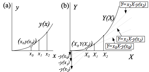
Fig. 12.8 Legendre contact transform S(x,y:X,Y) maps each point (xk, yk) to a contact point (Xk,Yk).
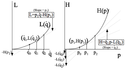
Fig. 12.9 Summary sketch of Legendre-Lagrangian-Hamiltonian geometry of Fig. 12.3 and 12.4.
The Equations of the Classical Universe (Lagrange, Hamilton, and others)
While
string theorists search for an “Equation of
the Universe”(EOTU) or a “Theory of Everything” (TOE) it should be noted that virtually all our
modern physics, however avant-garde, has a classical foundation in Lagrangian
or Hamiltonian equations. So a derivation of these all-important equations is
in order. We already have deduced, mostly by symmetry and functional trickery,
half of the Lagrange equations (![]() in 12.12c) and half of the Hamilton equations (
in 12.12c) and half of the Hamilton equations (![]() in 12.12d)
for purely kinetic quadratic form Lagrangian
in 12.12d)
for purely kinetic quadratic form Lagrangian![]() or
Hamiltonian
or
Hamiltonian![]() .
Needed now are the other half that add a potential energy U(x)
with spatial coordinate-x dependence to
.
Needed now are the other half that add a potential energy U(x)
with spatial coordinate-x dependence to ![]() and
and ![]() . That
wrecks our nice translational symmetry and momentum conservation. Fortunately,
the halves we have so far still apply. (Nature is so kind!) Also, the
to-be-derived EOTCU (Equations of the Classical
Universe) translate easily to “quite queer” coordinates {q1, q2,...} such
as polar, parabolic, hyperbolic, etc.
that were introduced in Ch. 10 in connection with complex potential
fields.
. That
wrecks our nice translational symmetry and momentum conservation. Fortunately,
the halves we have so far still apply. (Nature is so kind!) Also, the
to-be-derived EOTCU (Equations of the Classical
Universe) translate easily to “quite queer” coordinates {q1, q2,...} such
as polar, parabolic, hyperbolic, etc.
that were introduced in Ch. 10 in connection with complex potential
fields.
Generalized curvilinear coordinate (GCC) qm systems are a big deal with a long history coming after (de)Cartesian coordinates xj (or xj) introduced in Chapter 1. GCC superscript qm convention that puts the index m up (where exponents usually go) and its notation by letter-q may seem, well, quite queer. But, such oddity can be forgiven if the qm let us write all EOTCU in a single compact translatable form! It is based on an N-dimension differential chain relation between Cartesian coordinate (CC) differential dxj and GCC dqm.
![]() (12.18)
(12.18)
An N-dimension sum is implied over any index repeated (like m above) to avoid writing “Sigma”-sums.
An
identical linear relation exists between CC velocity ![]() and GCC
velocity
and GCC
velocity![]() .
.
![]()
![]() (12.19)
(12.19)
Total time-derivatives of CC (Cartesian velocity) and GCC (Generalized velocity) are denoted as follows.
![]()
![]()
In (12.19) Jacobian Jmj matrix
gives each CCC differential ![]() or
velocity
or
velocity![]() in terms of GCC
in terms of GCC ![]() or
or
![]() .
.
![]() (12.20a)
(12.20a)
Inverse (so-called) Kajobian Kjm matrix is defined by a partial derivative that is a flip of the one for Jmj.
![]() (12.20b)
(12.20b)
Product of
matrix Jmj and Kjm is a j-sum or
![]() that by definition
of partial derivatives, gives unit matrix.
that by definition
of partial derivatives, gives unit matrix.
![]()
So a Kjm matrix gives GCC ![]() or
or ![]() in terms of
in terms of ![]() or
or ![]() ,
respectively, the reverse of (12.18) or (12.19).
,
respectively, the reverse of (12.18) or (12.19).
![]()
![]()
GCC
acceleration or 2nd time-derivatives are a bit more
complicated. We first apply ![]() to
velocity (12.19).
to
velocity (12.19).
![]()
Then a
differential chain sum is applied to the Jacobian. Partial derivatives ![]() and
and ![]() are
reversible.
are
reversible.
![]()
Velocity
eq. (12.19) then equates total t-derivative of Jacobian to a partial qm-derivative
of CC velocity![]() .
.
![]() (12.21)
(12.21)
This and (12.20) are two main keys to converting the Newton Second Law (Newt II) to GCC forms that apply to all classical mechanical phenomena due to any number of particles in one, two, or three dimensions. These then serve as mathematical analogies or analogs to modern physics of relativity and quantum theory that describe optical, nuclear, atomic, and molecular phenomena that involve bizarre wavelike behavior in unimaginably countless dimensions. Even LHC physics is glimpsed but that’s still a work in progress.
Lagrange’s version of Newt-II (f=Ma)
Lagrange’s derivation starts with the following multidimensional CC version of Newt-II (f=Ma).
![]() (12.22)
(12.22)
It is based
upon a multidimensional CC version of kinetic energy that generalizes ![]() in (12.8).
in (12.8).
![]() (12.23)
(12.23)
Into the CC
expression for differential work ![]() is put
the 1st GCC differential (12.19).
is put
the 1st GCC differential (12.19).
![]() (12.24)
(12.24)
The dqm-sum is true term-by-term since dqm are independent. (Sum still holds if all dqm are zero but one.) This gives an expression for each generalized GCC force component Fm defined as follows.
![]() (12.24a)
(12.24a)
![]() (12.24b)
(12.24b)
Now for
Lagrange’s clever end game. First set![]() and
and ![]() with
with ![]() to
get:
to
get:
![]()
Then convert ![]() to
to ![]() by
(12.20a) on 1st
term and (12.21) on 2nd
term. Simplify by:
by
(12.20a) on 1st
term and (12.21) on 2nd
term. Simplify by:![]()
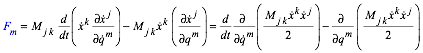
The result is Lagrange’s GCC force equation using kinetic energy (12.23).
![]() where:
where: ![]() (12.25a)
(12.25a)
But,
Lagrange isn’t done yet! If the force is conservative it’s a gradient ![]() or in GCC:
or in GCC:![]() .
.
![]()
This gives Lagrange’s GCC potential equation with a new definition for the Lagrangian: L=T-U.
![]() where:
where: ![]() (12.25b)
(12.25b)
Note that the potential function U cannot have any velocity ![]() dependence
or else the first term of (12.25b) would be wrong. Lagrange’s equations have
simple forms that use GCC momentum pm.
dependence
or else the first term of (12.25b) would be wrong. Lagrange’s equations have
simple forms that use GCC momentum pm.
![]() (12.25c)
(12.25c)
![]() (12.25d)
(12.25d) ![]() (12.25e)
(12.25e)
The first one (12.25d) is what we did not have when we found in (12.12c) the form ![]() . The latter is the CC version of
(12.25e) above. Pretty nice EOTCU (Equations
of the Classical Universe) here!
Let’s try them out.
. The latter is the CC version of
(12.25e) above. Pretty nice EOTCU (Equations
of the Classical Universe) here!
Let’s try them out.
Consider an example of Lagrange equations in polar coordinates (q1 = , q2 = ö) defined as follows.
x =x1= cos ö , y=x2 = sin ö
First we find Jacobian and Kajobian matrices. <J> is easy to get by (12.20a). Inverting <J> gives <K>.
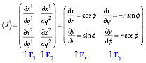
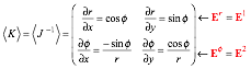 (12.26)
Two kinds of quasi-unit
vectors show up. Columns of <J> are covariant vectors ![]() and
and ![]() Rows
of <K> are contravariant
vectors
Rows
of <K> are contravariant
vectors ![]() and
and ![]() . They are
plotted and sketched generically in Fig. 12.10.
. They are
plotted and sketched generically in Fig. 12.10.
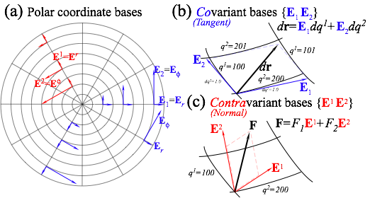
Fig. 12.10 Covariant force vector components in a polar space ( Eñ,Eö ).
Covariant vector ![]() is tangent to the qm coordinate
line of a cell wall.
is tangent to the qm coordinate
line of a cell wall. ![]() grows as its cell grows according to the 1st
differential relation (12.18) sketched in Fig. 12.10b and rewritten here in
vector notation.
grows as its cell grows according to the 1st
differential relation (12.18) sketched in Fig. 12.10b and rewritten here in
vector notation.
![]() (12.27)
(12.27)
Note ![]() grows in
Fig. 12.10a.
grows in
Fig. 12.10a. ![]() are
convenient bases for extensive
quantities like distance and velocity.
are
convenient bases for extensive
quantities like distance and velocity.
Contravariant vector ![]() is normal to the qm=const. surface or coordinate line of a
cell wall.
is normal to the qm=const. surface or coordinate line of a
cell wall. ![]() shrinks as its cell side grows according to
gradient relation (12.28) sketched in Fig. 12.10c.
shrinks as its cell side grows according to
gradient relation (12.28) sketched in Fig. 12.10c.
![]() (12.28)
(12.28)
![]() are
convenient bases for intensive
quantities like force and momentum.
are
convenient bases for intensive
quantities like force and momentum.
Polar
coordinates are orthogonal, but GCC ![]() and
and![]() are at home
in more exotic non-orthogonal manifolds and provide mutually orthonormal dual
bases with GCC orthogonality relations. (Prove this!)
are at home
in more exotic non-orthogonal manifolds and provide mutually orthonormal dual
bases with GCC orthogonality relations. (Prove this!)
![]() (12.30a)
(12.30a)
Scalar products ![]() •
•![]() give covariant metric
gmn-tensor matrix and similarly
give covariant metric
gmn-tensor matrix and similarly ![]() •
•![]() gives contra-gmn.
gives contra-gmn.
![]() (12.30b)
(12.30b) ![]() (12.30c)
(12.30c)
GCC
version for 1-free-particle Lagrangian ![]() involves gmn
factors using (12.27) and (12.30b).
involves gmn
factors using (12.27) and (12.30b).
![]() (12.31)
(12.31)
Polar coordinate metric tensors follow from (12.26). gmn and gmn are diagonal (orthogonal) mutual inverses.
![]()
![]()
The resulting polar-coordinate Lagrangian and its covariant momentum pm expressions (12.25e) follow.
![]()
![]()
![]() (12.32)
(12.32)
![]() is radial linear momentum.
is radial linear momentum.![]() is angular
momentum complete with moment of inertia
is angular
momentum complete with moment of inertia![]() . A
potential
. A
potential ![]() turns
the Lagrangian into
turns
the Lagrangian into ![]() of
(12.25b). Momentum t-derivatives (12.25d) follow.
of
(12.25b). Momentum t-derivatives (12.25d) follow.
![]()

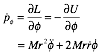 (12.33)
Note
how centrifugal force ![]() and
Coriolis force
and
Coriolis force ![]() are
derived so easily by Lagrange GCC. Also, if potential is radial-isotropic (no
are
derived so easily by Lagrange GCC. Also, if potential is radial-isotropic (no ![]() -dependence)
then angular momentum is a conserved constant.
-dependence)
then angular momentum is a conserved constant.
![]() (12.35)
(12.35)
Lagrange GCC is elegant and powerful. So is Hamiltonian GCC and, as we’ll see, it’s more conservative!
Hamilton’s version of Newt-II (f=Ma)
A GCC Hamiltonian H(p,q) uses momenta and coordinates as independent variables
rather than generalized velocities and coordinates employed by Lagrangian![]() . The total time derivative of L is
. The total time derivative of L is
![]() .
.
Here we leave open the possibility that the Lagrangian may have explicit time dependence and a non-zero partial t-derivative. (Think of a mad scientist dialing up the force field as the experiment progresses.)
The
Lagrange equations (12.25) let us insert momentum ![]() and its time
derivative
and its time
derivative ![]() into
(12.36).
into
(12.36).

A derivative identity![]() lets us
collect the two pq terms. Reordering gives a total t-derivative of a GCC version of a form (
lets us
collect the two pq terms. Reordering gives a total t-derivative of a GCC version of a form (![]() ) first
encountered in (12.11b). That’s the GCC Hamiltonian H(p,q).
) first
encountered in (12.11b). That’s the GCC Hamiltonian H(p,q).
![]() (12.36a)
(12.36a)
The momentum side (12.12) of Hamilton’s equations follows. So does the other (coordinate) side (12.36c).
![]() (12.36b)
(12.36b) ![]() (12.36c)
(12.36c)
To
get (12.36b) we apply![]() to H. (Recall
to H. (Recall ![]() =0.) To get (12.36c) we apply
=0.) To get (12.36c) we apply![]() to H. (Recall
to H. (Recall ![]() (12.25d).)
(12.25d).)
The Hamiltonian function has an unusual property. Its total time derivative equals its partial time derivative. If H lacks explicit time dependence it is a conserved constant. (Imagine our mad scientist asleep at the dial!) That constant is energy. To show this, apply metric definition (12.31) of T in L=T-U.
![]() (12.37a)
(12.37a)
![]()
![]() (12.37b)
(12.37b)
![]()
![]() (12.37c)
(12.37c)
So, the Hamiltonian is the sum of kinetic energy T and potential U which is the total energy E=T+U. Equations (3.12.5) amount to the conservation of total energy if L and H are not explicit functions of time.
Note
that we use the covariant
metric gmn
for the velocity v-dependent
Lagrangian, but the inverse contravariant metric gmn comes into play for the momentum p-dependent
Hamiltonian. Seem like so much formalistic foo-foo? Perhaps. But, just wait
until Unit 2 where we develop the relativistic and quantum mechanical versions
of this. Then this “formalism” will morph into the most sublimely gorgeous
geometry that you have ever imagined!
Variational calculus of Lagrangian mechanics
Here is a funny way to derive Lagrange’s equations. It involves something called variational calculus.
Variational calculus finds extreme (minimum or maximum) values to entire integrals such as
![]() (12.38)
(12.38)
Here
the curve q(t) can vary at each time t. If S(q) was a simple function like S(q)=q2 -4q we would find zeros of its derivative dS/dq =(2q-4)=0 at q=2 and be done. However, here S(q) is a functional,
that is, a function ![]() of
entire functions q(t) and t-derivative
of
entire functions q(t) and t-derivative
![]() either
of which can be varied arbitrarily at any point between limits t0 and t1 of the dependent time integration variable as shown in Fig.
12.11. (Again, we allow the possibility that
either
of which can be varied arbitrarily at any point between limits t0 and t1 of the dependent time integration variable as shown in Fig.
12.11. (Again, we allow the possibility that ![]() may
have explicit t-dependence, too.)
may
have explicit t-dependence, too.)

Fig. 12.11 Variation of functional
curve or trajectory path from q(t) to ![]()
An
arbitrary but small variation function ![]() is allowed
at every point t in the figure along the curve except at
the end points t0 and t1. There we demand it not vary at all.
is allowed
at every point t in the figure along the curve except at
the end points t0 and t1. There we demand it not vary at all.
![]() (12.39)
(12.39)
The
variant ![]() changes
integral (12.38) according to a first order Taylor series.
changes
integral (12.38) according to a first order Taylor series.
![]() (12.40)
(12.40)
Replacing ![]() with
with ![]() gives
a sum of two and then three integrals.
gives
a sum of two and then three integrals.
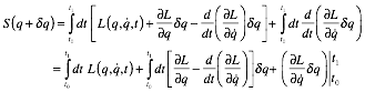
The third term vanishes according to (12.40). This leaves the following first order variation äS.
![]()
If integral S is an extremum its first order variation äS must be zero for all äq(t) even the case where äq(t) is only non-zero at only one tiny t-interval. Thus the äS integrand must be zero everywhere.
![]() (12.41a)
(12.41a)
The result is an Euler-Lagrange equation. It is a 1-dimensional version of GCC Lagrange equation (12.25c)
![]() (12-41b)
(12-41b)
We may just as well demand extreme (actually minimum) values for multi-dimensional Lagrange integrals.
![]() (12.38)N-dim
(12.38)N-dim
The result is the N-dimensional Lagrange equations (12.25) derived from Newt-II. But, why should Newt-II make the integral of Lagrangian minimum? Something weird underlies classical laws! Henri Poincare recognized early on that a new physics (modern physics) must be hiding down there.
Poincare’s invariant, quantum phase, and action
The
Legendre relation (12.11a) becomes Poincare’s
invariant differential if ![]() has dt
cleared.
has dt
cleared.
![]() (12.42a)
(12.42a)
It is also
the time differential dS of action ![]() whose
time derivative is rate L of quantum phase.
whose
time derivative is rate L of quantum phase.
![]() (12.42b)
(12.42b)
In Unit 2
we find DeBroglie law ![]() and
Planck law
and
Planck law![]() that,
if conserved, give a quantum plane wave:
that,
if conserved, give a quantum plane wave:
![]() (12.42c)
(12.42c)
Time-independent or Hamilton’s reduced action is the spatial integral ![]() . Classical
trajectories minimize action integrals S
and SH according to Least Action Principles like (12.41).
. Classical
trajectories minimize action integrals S
and SH according to Least Action Principles like (12.41).
Huygen's principle: "Proof" of classical axioms and path integrals
Enveloping curves generated by contact transformations like (12.15) or Fig. 12.7 are closely related to Huygen's principle of wave optics. This also applies to quantum waves of matter. Suppose a hypothetical action function SH(r0 : r) generates the curves SH(r0 : r)=10, 20, and 30 as sketched in Fig. 12.12.
Now imagine the same generator acts starting from two points r10 and r'10 on the SH(r0 : r)=10 wave front thereby generating two sets of intermediate wave fronts: SH(r10 : r)=10 and SH(r'10 : r)=10 around each of these two points. All points on these curves represent a total accumulation of 20 J.s of action since leaving r0, but only for select points like r20 and r'20 is 20 J. the least action that can be accumulated after leaving r0. All other points have a more direct route from r0 that is cheaper than 20 J.s.
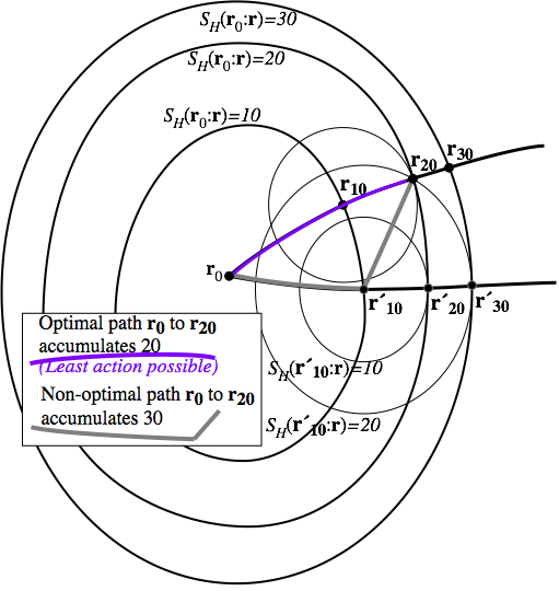
Fig. 12.12 Comparison of paths and wave fronts for discussion of Huygen's principle.
These special points r=r20 and r=r'20 of least action are just the contacting ones that lie on the envelope curve SH(r0 : r)=20. They also lie on optimal (least action) trajectory paths from r0 which have never failed to follow the undeviating "straight-and-narrow" paths determined by Lagrange equations. What makes these paths appear to follow the classical Lagrange equations? Why do they appear to optimize their action so faithfully? Huygens knew the answer in the 1600's, at least for rays of light. The key word here is "appear" since neither light waves nor matter waves originally have any intention of following a straight and narrow path!
Quite the contrary, every point on a Huygen's wave front broadcasts a continuum of deviant wave fronts in the form of the intermediate "wavelet" ovals such as SH(r10 : r)=10 and SH(r'10 : r)=10 in Fig. 12.12. But, for each of these non-optimal deviant "rascals" there are thousands more neighboring "rascals" whose actions vary linearly with deviation so that non-extreme action paths end up canceling each other by destructive interference of the varying phases due to deviant actions. No honor amongst "rascals" here!
Only for those optimal paths of stationary action (and therefore, stationary phase) do the phases add constructively, and it is only for these that quantum wave intensity or classical presence appears to exist most of the time in a classical world of enormous action. All paths are possible to varying degrees and exist in some sense, but only the optimal ones make their presence known and generally do so while obeying quite precisely the classical equations of motion.
In a sense, this constitutes an evolutionary proof of Newton's "laws" or at least justification of Newton's axioms in the case of high action or the classical limit. The classical world appears to be a result of a continual process of natural selection!
However, the situation is different for systems with discrete or limited number of paths as in the case of low action or when wavelength is comparable to the size of a system. Then the classical myth is likely to disintegrate like Dracula out of his coffin at dawn! Now matter how dearly we believe in our precisely machined gears and fine particles there comes a time and place where the classical equations part company with new reality that appears with increasingly clever and precise experimental evidence.
Nevertheless, the classical apparatus is far too well developed to die forever, and it rises to assist the newly appointed quantum paradigm in what is called semi-classical approximation theory. The role of generating action functions S(r0,t0 : r,t) and SH(r0 : r) is taken over in quantum theory by amplitudes, wavefunctions, or matrix elements such as the amplitude 〈r,t| r0,t0〉 of time-evolution and or the transition-overlap amplitude 〈r | r0 〉. Here, |〈 B | A 〉|2 is the probability for a state-A to become state-B if forced to make a choice. Bracket 〈 B | A 〉 is called a probability amplitude; past-to-future is read right-to-left like Hebrew. Probability amplitudes may be approximated by semi-classical relations similar to (12.42c).
![]() (12.43a)
(12.43a) ![]() (12.43b)
(12.43b)
Restating Huygen's principle with semiclassical amplitudes gives a completeness or closure relation.
![]() (12.44)
(12.44)
Intermediate r'-path sums, as in Fig. 12.12, cancel by phase variation except on the optimal stationary-action path r1←r0. The sum over phase factors from r'-paths is well approximated by the amplitude for the stationary optimal path. Methods for summing over all paths of significant importance (including deviant ones) are called Feynman path integration techniques. This is a difficult chore since “all paths...” are a tangled uncountably infinite mess. Often, the extra effort needed to count them is not needed.
Bohr quantization
requires quantum phase ![]() in
amplitude (12.44) to be an integral multiple õ of 2π after a
closed loop integral
in
amplitude (12.44) to be an integral multiple õ of 2π after a
closed loop integral ![]() .
The integer õ (õ =
0, 1, 2,...) is a quantum number.
.
The integer õ (õ =
0, 1, 2,...) is a quantum number.
![]() (12.45)
(12.45)
A colorful way to display action and its Bohr quantization is to numerically integrate Hamilton's equations and Lagrangian L and color the trajectory according to the current accumulated value of action.
SH(0 : r) = Sp(0, 0 : r, t ) +
Ht =![]() + Ht . (12.46)
+ Ht . (12.46)
The hue should represent the phase angle SH(0 : r)/h modulo 2π as, for example, 0=red, π/4=orange,
π/2=yellow, 3π/4=green, π=cyan (opposite of red), 5π/4=indigo, 3π/2=blue, 7π/4=purple, and 2π=red (full color circle). Interpolating action on a palette of 32 colors is enough precision for low quanta.
The colored paths display a confused gray mess if phases fail to interfere constructively. But, for select quantizing values of energy, there appear striking patterns of colors when Bohr quantization makes phases interfere constructively. Patterns are outlines of spatial quantum wave amplitudes (12.43b).
![]() (12.43)repeated
(12.43)repeated
This color-quantization technique was done on a CRAY-Dicomed film system by Heller and Davis in 1983.
A
quantizing example for a 2-dimensional oscillator using the ColorU(2) program is shown in Fig. 11.13. Viewing
this in gray-scale is possible since only two hues actually survive: red, representing a phase of 0, and cyan,
representing a phase of π. The example is a standing wave mode in (x,y)-coordinate space, so the only possible
wave amplitude is ±1, that is, complimentary hues red and cyan which appear as light and dark gray in a gray scale
portrait. Remaining colors pile up on nodal lines with so many phases
interfering to destroy the amplitude. A time-dependent action S(0,
0 : r, t ) (12.43a) gives time-dependent moving waves such as the
snapshot in Fig. 11.14 of a quantum fountain discussed after Fig. 12.5. Wave
animation is done by shift the computer color wheel by the time-dependent phase
angle ![]() in
(12.46).
in
(12.46).
![]() (12.46)
(12.46)
A moving wave has a quantum phase velocity found by setting S=const. or dS(0,0:r,t)=0=p•dr-Hdt .
![]() (12.47)
(12.47)
This is quite the opposite of classical particle velocity which is quantum group velocity.
![]() (12.48)
(12.48)
By making two of the entries in the phase-color palette to be black-and-white it is possible to display a wave front line which will march in step with the other hues in the palette.

Fig. 12.13 Phase-color 2-dimensional harmonic oscillator paths showing (2,2) quantum wave function.
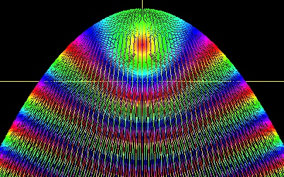
Fig. 12.14 Phase-color trajectory paths showing quantum wave fronts of moving wave.
A sequence of quantum wavefronts underlying the quantum fountain are drawn in Fig. 12.15 for three different values of reduced action SH. This is equivalent to taking snapshots at different times. As classical momentum approaches zero at the top of Fig. 12.15b, the S wave phase speed diverges to infinity. Then two "cat ears" are created and race out along the top of the classical envelope in Fig. 12.15c and then slow down as the classical momentum p again picks up. High p in Fig. 12.15 means high gradient ∇SH = p so the SH contours are closer together. S fronts move from one SH =n2π contour to the next SH =(n+1)2π contour at frequency ù=H/h so large p means slow going. Note that the lower regions of each contour in Fig. 12.15 are slower than upper regions; quite the opposite of the classical particle “ball” in Fig. 12.5. The two "cat ears" move out and down rapidly until, like Lewis Carroll's Cheshire cat, nothing remains but its smile!
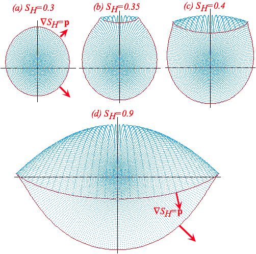
Fig. 12.15 Constant SH contours for iso-energetic trajectory family are normal to trajectory paths.
Dynamics of phase and group velocity are the key to relativity and quantum theory as Unit 2 will show.
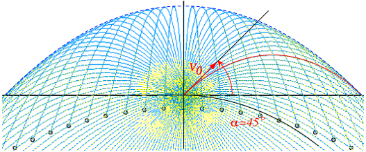
The volcanoes of Io and NIST atomic fountain
1.12.1. A fountain spraying water in many directions at equal speed appears to form a parabola of revolution whose cross-section is plotted above. You see this also in photos of volcanoes on Jupter’s moon Io. Let’s model this with a Bang! of equal-initial-speed v0 particles ejected from origin in uniform gravity g vacuum and develop geometry of parabolic trajectories and their envelope. Key questions: “What curve or “blast wave” do the particles form at each moment of time?” and “Is the envelope, in fact, parabolic?”
(a) First describe how observers see the trajectories behave if they are riding in a well-shielded free-falling elevator frame-(x´,y´) that passes the origin point at the moment of ejection.
(b) Meanwhile, in the lab (x,y)-frame, describe the parabolic fragment trajectories as a function of the initial elevation angle á for each fragment. Give equations for the focal point of each parabola and describe what curve these foci form (the focus-locus). (See if you can do it without peeking at Ch. 12.)
(c) Construct examples of parabolas with their focus-locus and find a relation between the focal point and the contact point for each parabolic path with the envelope. Is the envelope parabolic? and, if so, where is its focus? Construct drawings of á =30° and á =45° paths and “blast wave” at the moment each path contacts the envelope.
Problem for a volcanolgist (or baseball outfielder)
1.12.2. Suppose you are on the x-axis some distance from the origin where a baseball (or volcano rock) is thrown up and toward you so it appears to move straight up the y-axis like an imaginary elevator that is at the line-of-sight projection of baseball (or rock) onto y-axis. Elevator motion indicates if you are in position to catch the ball (or be clobbered by the rock) or whether the object will fly over or fall short. Describe apparent elevator velocity and/or acceleration that distinguishes the three cases, particularly the middle one.
1.12.3.
Suppose a neutron starlet enters a pocket of U235 at position r(0) and goes Bang!
The U235 detonates and blasts off pieces of starlet that each fly away
with the same initial speed |v(0)|=1 (we assume)
but various velocities v(0) =(0,1), (![]() ),
(0,1), (
),
(0,1), (![]() ), etc. (Units use the usual geometric ù=1
scaling.)
), etc. (Units use the usual geometric ù=1
scaling.)
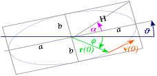
The short answer problems concern the resulting orbits of equal mass starlet pieces inside the Earth.
Do the starlet blast orbits conserve values for any physical quantities such as (Yes or No) initial
speed |v|?__, momentum |p|?__, angular momentum l?__, KE?__, PE?__, total Energy E?__ .
Do the starlet blast orbits conserve values for some geometric quantities such as (Yes or No)
a?__, b?__ , r?__ , H?__, ö?__, ϑ?__, á?__. (See sketch of general ellipse orbit above.)
For whichever it is possible, give |v|, |p|, l, KE, PE, or E in terms of a, b, H, ϑ or á. Note if any correspond to particular geometrical length or area that characterizes an orbit.
Do the starlet blast orbits share equal values for any physical quantities such as (Yes or No)
Average momentum p?__, angular momentum l?__, average KE?__, average PE?__, total E?__ .
Do the starlet blast orbits share equal values for some geometric quantities such as (Yes or No)
a?__, b?__ , H?__, ö?__, ϑ?__, á?__. (See sketch of general ellipse orbit above.)
Geometric orbit and envelope constructions
Using the graph on the attached page, do the following for initial position vector r(0) =(1,0):
(a) Construct the orbit for initial v(0) =(0,1) in part (a) of the graph.
(b) Construct the orbit for initial v(0) =(1,0) in part (b) of the graph.
(c)
Construct the orbit for initial v(0) =(![]() ) in part (c) of the graph.
) in part (c) of the graph.
(d)
Construct the orbit for initial v(0) =(![]() ) in part (c) of the graph.
) in part (c) of the graph.
(e) There is a “blast wavefront” or locus of starlet pieces that expands with each instant of time. Using whatever means you like, plot points of this curve for t/ôperiod= 1/12, 2/12, 3/12, and 4/12.
(f) There is a constant contacting curve that envelops all orbits with r(0)=(1,0) and |v(0)|=1.
Construct this enveloping boundary for |v(0)|=1. How does the envelope vary with initial speed |v(0)| ?
(g) See if you can deduce a relation between the focal point(s) and the contact point(s) for each elliptic path with the envelope. Is the envelope also elliptic? If so, where are its foci?
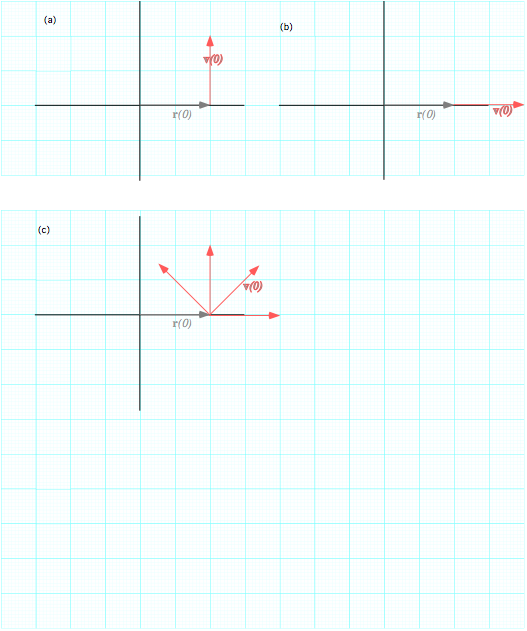
Appendix 1.A Vector product geometry and Levi-Civita åijk
Vectors have relative projections onto each other. Components x, y, or z
are projections of r onto unit i, j, and k. Power F•v
=Fvcosè is a dot product cosine projection of F on v. Coriolis a=![]() =wvsinè is a sine-like transverse projection
called the cross
product. Product A•B (or |AxB|) is cosine (or sine) of a relative
angle (èB-èA) times length factor AB shown in Fig. 1.A.1. Also, recall
complex products in (10.30).
=wvsinè is a sine-like transverse projection
called the cross
product. Product A•B (or |AxB|) is cosine (or sine) of a relative
angle (èB-èA) times length factor AB shown in Fig. 1.A.1. Also, recall
complex products in (10.30).
The cosine or dot-projection may be given in Cartesian lab components (Ax=AcosöA) Ay=AsinöA).
![]() (1.A.1a)
(1.A.1a)
The sine or cross-projection has a somewhat different or “crossed-up” form.
![]() (1.A.1b)
(1.A.1b)
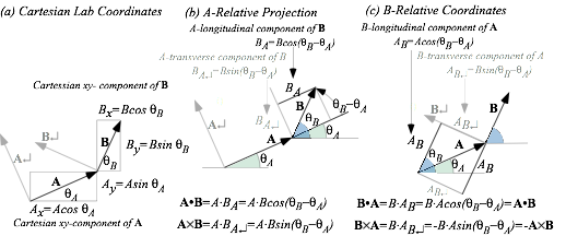
Fig. 1.A.1 Vector component geometry (a) Lab-relative. (b) A-relative. (c) B-relative.
Here A•B and AxB are numbers or scalars. Full AxB definition ((1.A.4b) below) is a vector perpendicular to both A and B. (In Fig. 1.A.1, it would stick out of the page.) Also it happens that AxB is the area of the vector parallelogram and 1/2AxB is the area of the A+B or A-B triangle as shown in Fig. 1.A.2.
In Fig. 1.A.1b vector B refers to axes made of vector A and its perpendicular copy A↵ and vice-versa in Fig. 1.A.1(c). Dot products are reflexive (A•B = B•A). However, cross products must be anti-reflexive (AxB =-BxA) since the B↵ vector is in a negative direction relative to A in Fig. 1.A.1(c). One way to display the relation between the pair (A, A↵) and the pair (B, B↵ ) is in a rotation matrix.
![]() (1.A.2)
(1.A.2)
Algebraic definitions of A•B and AxB are based on the symmetric Kronecker function äij and the totally anti-symmetric Levi-Civita function åijk defined as follows.
![]() (1.A.3a)
(1.A.3a)
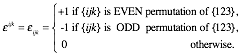 (1.A.3a)
These are fundamental to tensor analysis and exterior calculus that will be introduced in Unit 3.
They also define scalar A•B and vector AxB products in useful ways for fast computer logic, as follows.
![]() (1.A.4a)
(1.A.4a) ![]() (1.A.4b)
(1.A.4b)
The notation Ck=(C)k denotes the kth component of a vector C.
Determinants and triple products
Levi-Civita sums define the determinant detU of a matrix Uij. An expansion by minors is shown here.
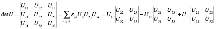 (1.A.5)
A triple vector product AxB•C is such a determinant made from a matrix of three vector components.
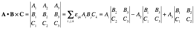 (1.A.6a)
![]() (1.A.6b)
(1.A.6b)
Minor expansion (1.A.5) is a (•)-product
of A with (![]() )-product
vector BxC. Base area |BxC| times altitude (A projected onto normal BxC) equals the parallelepiped volume
enclosed by A, B, and C.
)-product
vector BxC. Base area |BxC| times altitude (A projected onto normal BxC) equals the parallelepiped volume
enclosed by A, B, and C.
Anti-symmetric å-forms let us generalize geometry from 2-and 3-dimensions to N-dimensions. Advanced mechanics has many dimensions. One mole (6·1023 particles) has at least 6·1023 dimensions and two or three times that if the atoms move in 2D or 3D. So å-forms are necessary!
Products of anti-symmetric å-forms reduce to symmetric ä-forms by a LeviCivita identity.
![]() (1.A.7)
(1.A.7)
A triple-cross-product formula ![]() is a
first application.
is a
first application.
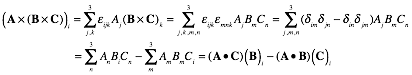
The LC-identity (1.A.7) reduces each sum over k to dot-product terms.
![]()
Fig. 1.A.2 Cross-product and area of (a)-(b) Parallelogram, (c) Sum triangle, (d) Difference triangle.
The Levi-Civita å-identity
is helpful for unraveling operator products. One example is the expressions for
magnetic force ![]() where
field B is a curl
where
field B is a curl ![]() of
vector potential A that occurs in Unit 2 Ch. 8.
of
vector potential A that occurs in Unit 2 Ch. 8.
![]()
Index notation for the double-cross
product is the following. Note å-symmetry gives:![]()
![]()
Here the dummy-index-convention sums any indices repeated on one side of the equation such as i, j, a, and b above. Applying the Levi-Civita å-identity reduces the equation.
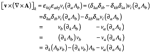
This is converted back to Gibbs’s bold vector notation that involves tensors like ![]() and
and ![]() .
.
![]()
Again, tensor index notation helps to
distinguish ![]() ,
,![]() , and
, and ![]() .
.


![]()
However, in Newtonian mechanics the
position ![]() and velocity
and velocity
![]() have no explicit dependence and so all r-partial derivative of v (or vice-versa) are identically
zero.
have no explicit dependence and so all r-partial derivative of v (or vice-versa) are identically
zero.
![]()
Then the double-cross product reduces as follows.
![]()
Try using å-identities to
reduce ![]() ,
, ![]() ,
, ![]() , and
, and ![]() .
.